Hardware-Aware Programming for Dummies!

Hardware-aware programming requires matching your computational task to the right processor architecture while aggressively minimizing data movement bottlenecks. While CPUs use large caches and complex logic to minimize latency for sequential tasks, GPUs use massive parallel arrays to maximize throughput for parallel workloads. However, the ultimate performance killer is data movement latency across the PCIe bus between the CPU and GPU; for small workloads, this transfer time completely eclipses the actual compute speed. Maximizing efficiency therefore relies on software-level optimization, such as avoiding warp divergence in GPU kernels so threads don't sit idle, and properly configuring PyTorch dataloaders with pinned memory and prefetching to keep the GPU continuously fed with data.
Foremost, let’s introduce the concept of vectorization, below are presented some comparative code examples. First step is to master the shift from iterative (scalar) logic to vectorized logic. While the following examples utilize NumPy on the CPU, the underlying principles of data parallelism are identical to those used in CUDA or Metal kernels.
In a standard loop, the Python interpreter must handle type-checking and list overhead for every single iteration. Vectorization offloads this to highly optimized C and assembly routines.
Iterative Approach (Scalar):
import time

# Multiplying two arrays of 1,000,000 elements
size = 1000000
a = list(range(size))
b = list(range(size))
result = []

start = time.time()
for i in range(size):
    result.append(a[i] * b[i])
Vectorized Approach (NumPy):
import numpy as np

a_np = np.arange(size)
b_np = np.arange(size)

start = time.time()
# The operation is dispatched to the CPU's SIMD units
result_np = a_np * b_np
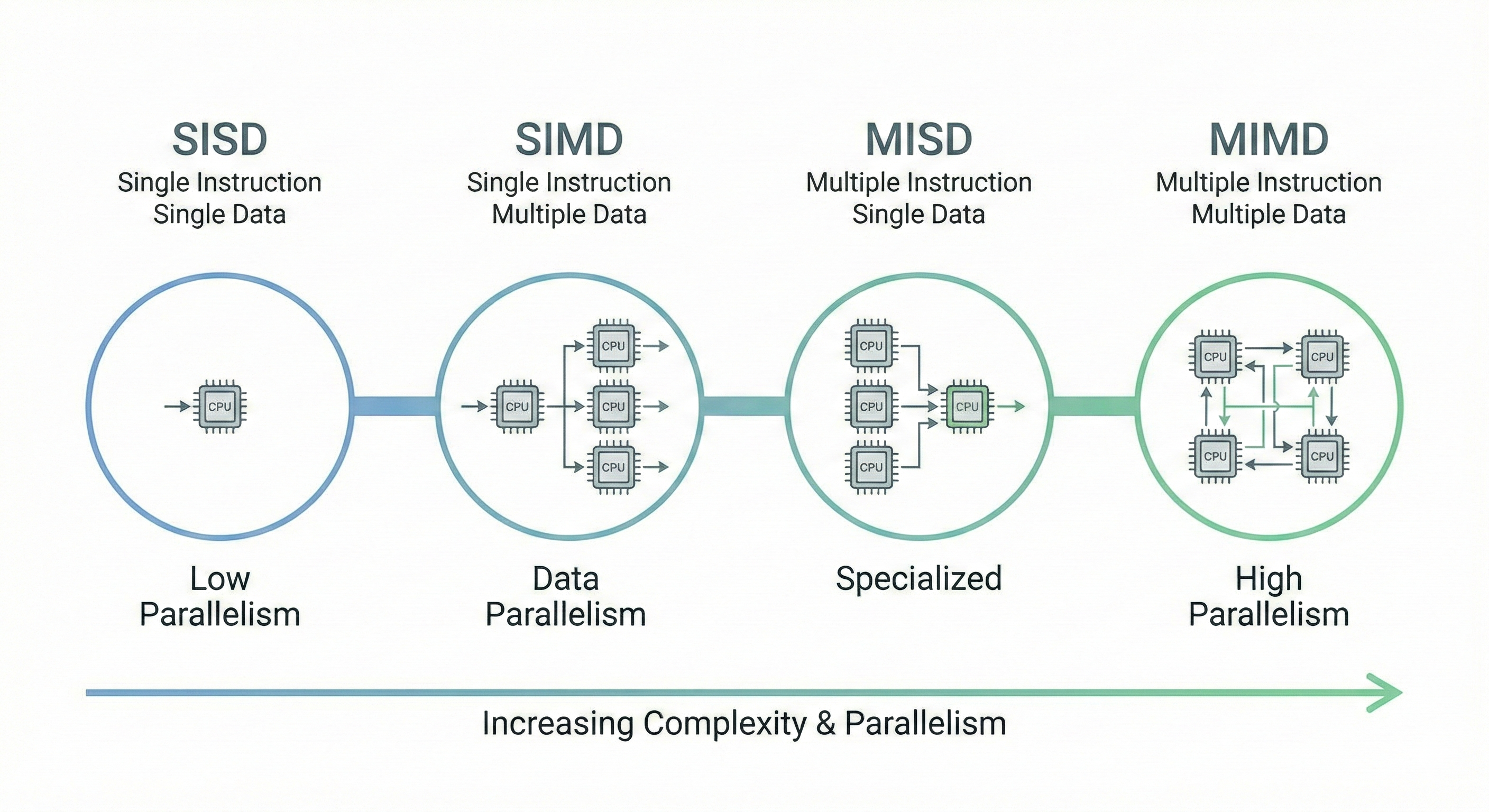
These examples illustrate how removing explicit loops allows the underlying library (NumPy) to utilize SIMD (Single Instruction, Multiple Data) instructions instead of SISD (Single Instruction, Single Data) which is the foundational mindset needed for hardware-aware programming. SIMD isn’t the only available paradigm, Flynn’s Taxonomy describes computer architectures based on the number of concurrent instruction and data streams.
Flynn’s Taxonomy Overview#
SISD (Single Instruction, Single Data stream)
- A single processor executes a single instruction stream to operate on data stored in a single memory.
SIMD (Single Instruction, Multiple Data stream)
- A single instruction is broadcast to multiple processing elements, each operating on different data points simultaneously.
MISD (Multiple Instruction, Single Data stream)
- Multiple instructions operate on the same data stream. This architecture is relatively rare in general computing and is typically used for fault tolerance or specialized digital signal processing.
MIMD (Multiple Instruction, Multiple Data stream)
- Multiple autonomous processors simultaneously execute different instructions on different data.
- Multiple autonomous processors simultaneously execute different instructions on different data.
What is a GPU?#
A GPU is a specialized parallel processor designed to perform rapid mathematical calculations, particularly those needed for rendering images, videos, and animations.
As you can sense, all the tasks mentioned before requires highly intensive parallel processing and indeed GPUs are optimized for parallel processing, so executing many operations simultaneously on different devices (the concept of devices will be cleared in the next sections), making algorithm optimized for GPU part of the family of MIMD computations.
The architectures for both CPU and GPU cores are illustrated in the figure below.
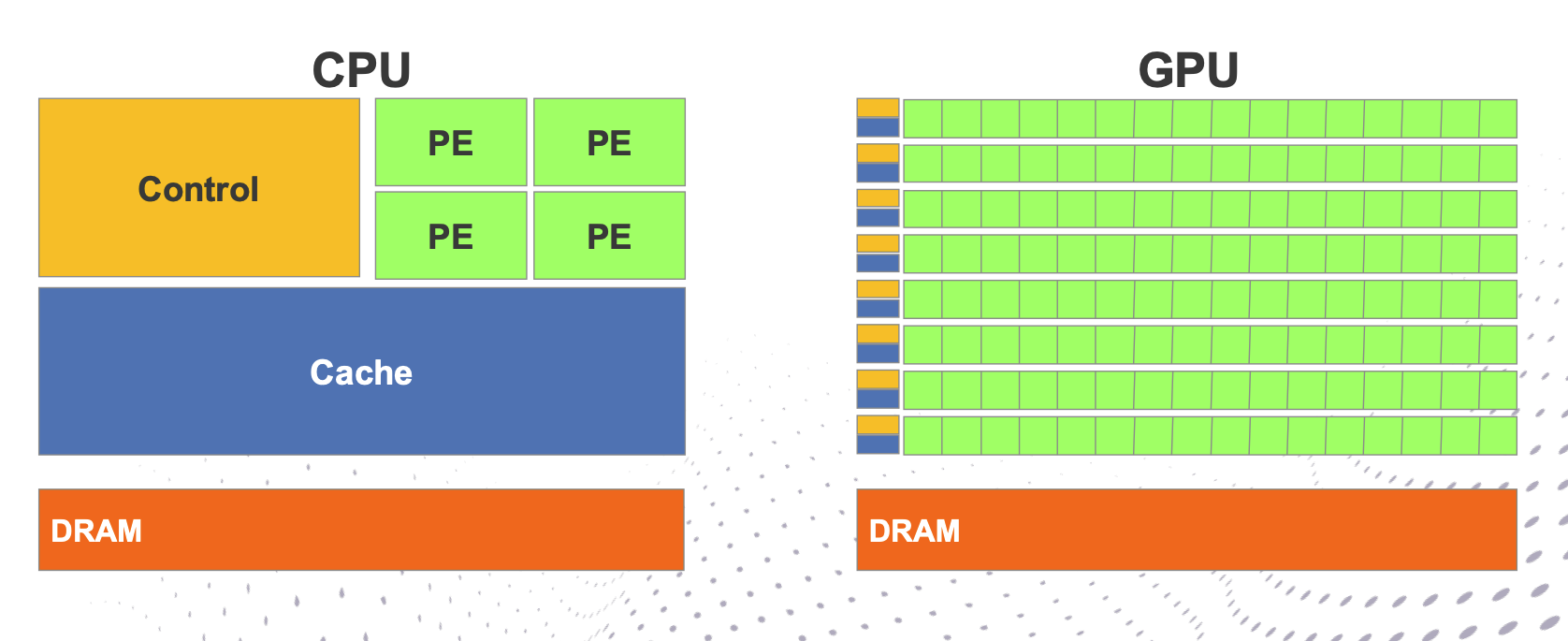
CPU hardware minimizes data processing latency by utilizing large caches and complex control logic. For instance, the internal hardware control logic is often significantly more convoluted than the linear sequence of instructions a programmer writes. Consequently, CPU technology drives optimization through techniques such as Branch Prediction and Out-of-Order execution, which specifically leverage Instruction Level Parallelism (ILP).
On the other hand, GPU hardware dedicates the majority of its silicon to Processing Elements (PEs) and registers, hiding memory and instruction latencies through massive parallel computing operations. Unlike CPUs, GPUs refrain from reordering operations; mechanisms like context switching and flow reorganization are inefficient for this architecture given the small caches available to thread blocks and the limited compute power per individual core.
The architecture of a modern GPU is defined by a hierarchical relationship between memory and compute units. At the base, the Global Memory—typically labeled as DRAM—serves as the primary storage hub, linked to multiple matrices of Processing Elements (PEs). In most standard architectural nomenclature, these matrices are referred to as Streaming Multiprocessors (SMs). Each SM operates as a self-contained unit, equipped with its own dedicated resources to manage localized workloads:
- Shared Memory: Facilitates high-speed data exchange between the PEs within a specific block.
- Registers: Provides the immediate, low-latency workspace required for active threads.
The specific count and dimensions of these components are dictated by the underlying architecture. Over the years, it is fair to say that these specifications have increased “just a bit”—evolving from modest parallel cores to the massive, high-density arrays we see in cutting-edge hardware today.
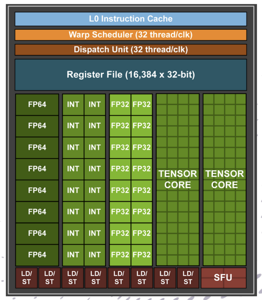
A low-level representation of the PE is then provided, illustrating how a single Processing Element is further decomposed into multiple sub-units, each dedicated to a specific computational task.
 Building on our architectural overview, we can see the sheer scale of evolution by comparing the Pascal P100 (the first to introduce HBM and NVLink) with the massive leap represented by the Ampere A100.
While both share a similar organizational philosophy, the “bit” of an increase mentioned earlier is actually a generational chasm in density and specialized throughput.
Building on our architectural overview, we can see the sheer scale of evolution by comparing the Pascal P100 (the first to introduce HBM and NVLink) with the massive leap represented by the Ampere A100.
While both share a similar organizational philosophy, the “bit” of an increase mentioned earlier is actually a generational chasm in density and specialized throughput.
| Feature | Pascal P100 (SXM2) | Ampere A100 (40GB) |
|---|---|---|
| Total SMs | 56 | 108 – 128 (Architecture Max) |
| FP32 Cores | 3,584 | 8,192 |
| INT32 Cores | N/A (Shared with FP) | 8,192 (Dedicated) |
| Tensor Cores | None | 432 (3rd Gen) |
| L2 Cache | 4 MB | 40 MB (10x Increase) |
| HBM2 Capacity | 16 GB | 40 GB |
| Memory Bandwidth | 732 GB/s | 1,555 GB/s |
| NVLink Bandwidth | 160 GB/s | 600 GB/s |
MFU (Model FLOPs Utilization)#
MFU is the ratio between the actual math our GPU performed, in terms of FLOPs in this case, and its theoretical peak performance.
$$\text{MFU} = \frac{\text{Achieved TFLOPS}}{\text{Peak TFLOPS for the Precision}}$$To test A100’s efficiency, we can benchmark a large square matrix multiplication ($C = A \times B$). This is the most “pure” way to test MFU because it minimizes the messy CPU overhead and focuses entirely on the GPU’s execution units.
Results#
Benchmarking torch.bfloat16 on NVIDIA A100-SXM4-40GB Matrix size: 8192x8192 | Theoretical Peak: 330 TFLOPS Avg Time: 4.37 ms Achieved: 251.81 TFLOPS MFU: 76.30%
Benchmarking torch.float32 on NVIDIA A100-SXM4-40GB Matrix size: 8192x8192 | Theoretical Peak: 19.5 TFLOPS Avg Time: 57.39 ms Achieved: 19.16 TFLOPS MFU: 98.26%
GPU Programming Basics#
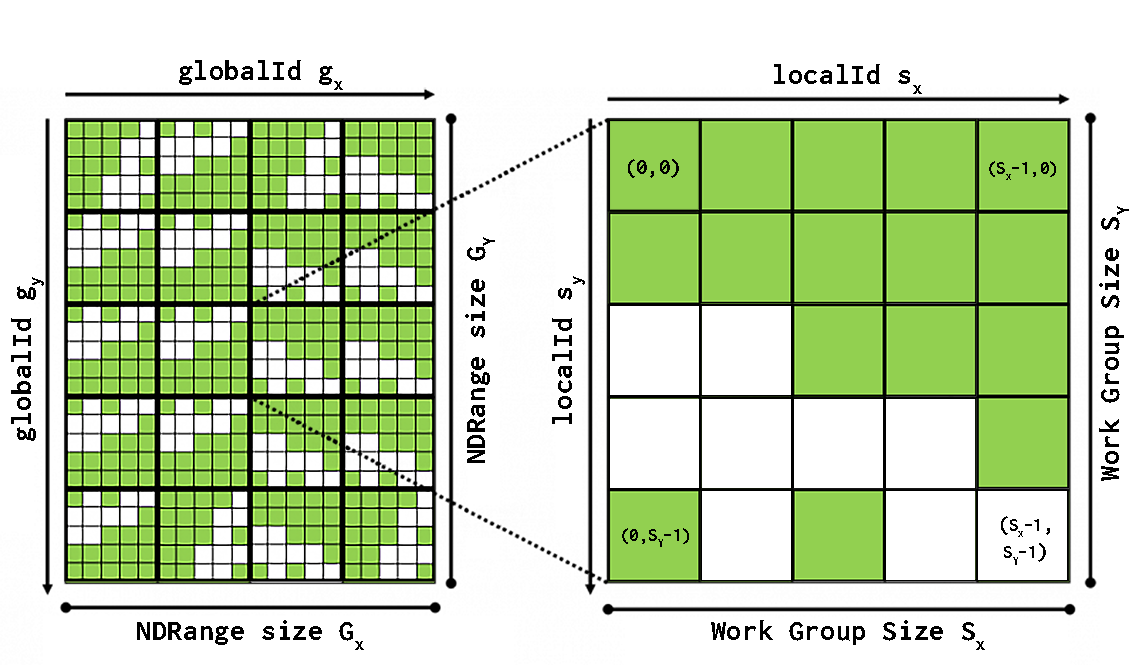
In order to abstract the underlying hardware, GPU programming presents a hierarchical structure at the software level. At the top of this hierarchy is the Grid, which represents the entire execution space for a specific Kernel. We will talk about kernels shortly; for now, think of them as the basic functions of GPU programming.
The Grid is further subdivided into Blocks (or Thread Blocks), which are groups of threads that can cooperate and share memory. On a hardware level, these blocks are partitioned into Warps—typically groups of 32 threads running in lockstep. This means every thread in that group (Warp) executes the exact same instruction at the exact same time.
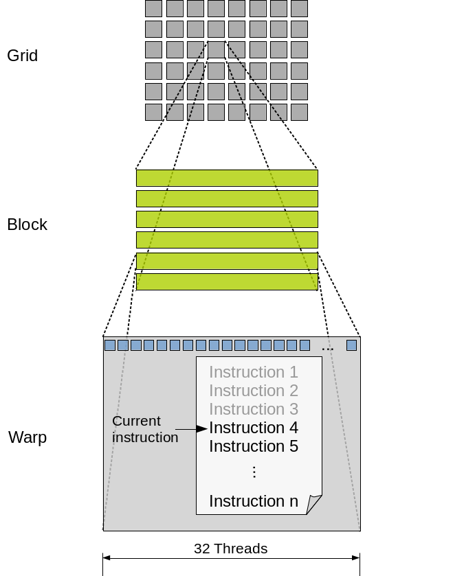
While physical memory is linear (1D), the grid—and its underlying structures—is often represented in a 2D or 3D arrangement. We can assign any dimensionality required to optimize the specific calculus of our task.
The Kernel#
If the Grid, Blocks, and Threads are the “workers,” the Kernel is the “set of instructions” given to every single one of them. In standard CPU programming, you might write a for loop that executes a function 1,000 times sequentially. In GPU programming, you write a Kernel once and launch it. The GPU then instantly spawns thousands of threads (the Grid), and every single thread executes that same kernel code simultaneously.
As you might have guessed, while every thread runs the same code, they don’t do the same work. They use the hierarchy defined in the kernel to determine their unique identity. The kernel is a template; it doesn’t know about your specific data (like “pixel 400” or “matrix row 5”) until it runs. It only knows logic.
Inside the kernel code, each thread looks at the hardware registers to calculate its unique Global ID:
- Which Block am I in? (
blockIdx) - Which Thread inside that block am I? (
threadIdx) - How big are the blocks? (
blockDim) The formula for the unique index is:
Warp Divergence#
When you launch the kernel, the hardware groups threads into Warps. If your kernel contains an if/else statement where half the threads in a Warp take the if path and the other half take the else path, they can no longer run in parallel. This is called Warp Divergence.
Because the Warp moves in lockstep, it must execute the if path while the else threads sit idle, and then execute the else path while the first group waits. This behavior can absolutely kill performance.
if (thread_id < 16) {
    do_A(); // First half of the warp does A, second half idles
} else {
    do_B(); // Second half does B, first half idles
}
A well-written kernel ensures that threads within the same Warp follow the same code path as much as possible.
Practical Implementation#
A typical kernel in CUDA C++ looks like this:
// THE KERNEL (The instruction sheet)
// The __global__ keyword tells the compiler this runs on the GPU.
__global__ void myKernel(float* data) {
    // IDENTITY: "Who am I in this grid?"
    int i = blockIdx.x * blockDim.x + threadIdx.x;

    // WORK: "I will process only the data at index i"
    data[i] = data[i] * 2.0f;
}

int main() {
    int N = 1024;
    int threadsPerBlock = 256;               // Block size
    int blocksPerGrid = N / threadsPerBlock; // Number of Blocks

    // Launch the Kernel: <<<Grid Size, Block Size>>>
    myKernel<<<blocksPerGrid, threadsPerBlock>>>(device_data);
}
Dimensionality and Memory#
We can structure grids in 2D or 3D to match the logical shape of our data. For example, if you’re applying a 3x3 convolution to an image, a 2D grid is a better fit. An image is inherently a 2D plane; using a 1D grid would require manual row/column calculations using modulo arithmetic, which is computationally expensive and hard to read.
@cuda.jit
def conv3x3_kernel(inp, out, k):
    # inp: HxW, out: (H-2)x(W-2), k: 3x3 kernel
    i, j = cuda.grid(2)
    H = inp.shape[0]
    W = inp.shape[1]
    out_H = H - 2
    out_W = W - 2
    if i < out_H and j < out_W:
        s = 0.0
        # apply 3x3 convolution
        for di in range(3):
            for dj in range(3):
                s += k[di, dj] * inp[i+di, j+dj]
        out[i, j] = s
Conversely, for a simple vector operation like SAXPY ($y = ax + y$), a 1D grid with a grid-stride loop is the most efficient approach:
@cuda.jit
def saxpy_kernel(x, y, a):
    i = cuda.grid(1)
    n = 10_000_000
    stride = cuda.gridsize(1)
    while i < n:
        y[i] += a * x[i]
        i += stride
Data Movement as a bottleneck#
However, the primary challenge in this architecture remains the data movement bottleneck. Because the GPU (Device) and the CPU (Host) have separate memory pools, performance is often limited by the speed of the PCIe bus.
To understand better how memory is arranged check memory hierarchy in the image below. This necessitates efficient management of data transfers, categorized as H2D (Host-to-Device) and D2H (Device-to-Host).
While H2H (Host-to-Host) and D2D (Device-to-Device) transfers also occur, the latency involved in moving data across the PCIe bus remains the most critical bottleneck for developers to optimize.
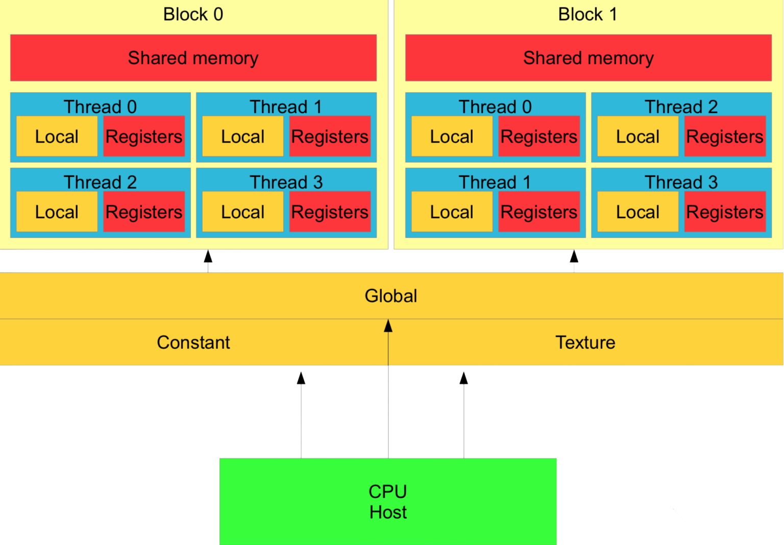
Of course, the lower we go in the hierarchy, the faster and smaller the memory becomes. Blocks share the same memory, so it makes sense to avoid communication between different blocks.
The same holds for GPU Global Memory and Central Memory on the CPU; the objective is always to avoid data movement. In an ideal case, we would have all the data we require in the right place at the right time.
PyTorch and Use Cases#
Maybe you’ve heard about this magic framework that lets you build the next SoTA LLM with zero effort, just by describing it in a Pythonic way. It sounds like a bargain. Well, like everything in computer science, it only seems that way.
PyTorch is just a very fine abstraction over a massive pile of C++ and CUDA code. Using PyTorch means triggering a dozen different lower-level frameworks all at once, completely oblivious to what you’re actually doing to the hardware during that never-ending epoch—which, looking at TensorBoard, is just going to result in a messy overfit anyway.
This simplified breakdown illustrates how PyTorch’s internal architecture actually processes a basic operation:
User Code: You type
z = x + yin Python and hit run. In reality, you are submitting a high-level work order to a low-level language.PyTorch Dispatcher: That central framework (c10) catches your code and instantly checks your tensors in order to route them to the suitable underlying backend.
CPU Backend: If you forgot to call
.to('cuda')—and let’s be honest, you probably did—the Dispatcher sends the job to libraries such as Intel’s MKL or oneDNN. They will give you a truly slow computation, but at the end of the day, they’re also software with emotions, so don’t bully them.GPU Backend: If you actually paid for an NVIDIA GPU, the Dispatcher hands the job off to cuBLAS or Triton, which will parallelize the math across thousands of cores, burning enough electricity to dim your neighborhood just so your loss curve can plateau faster.
Autograd Engine: If
requires_grad=Trueis enabled, this engine acts as a wiretap, aggressively logging every single operation into a massive computation graph. When you inevitably call.backward(), it can magically spit out the chain rule math.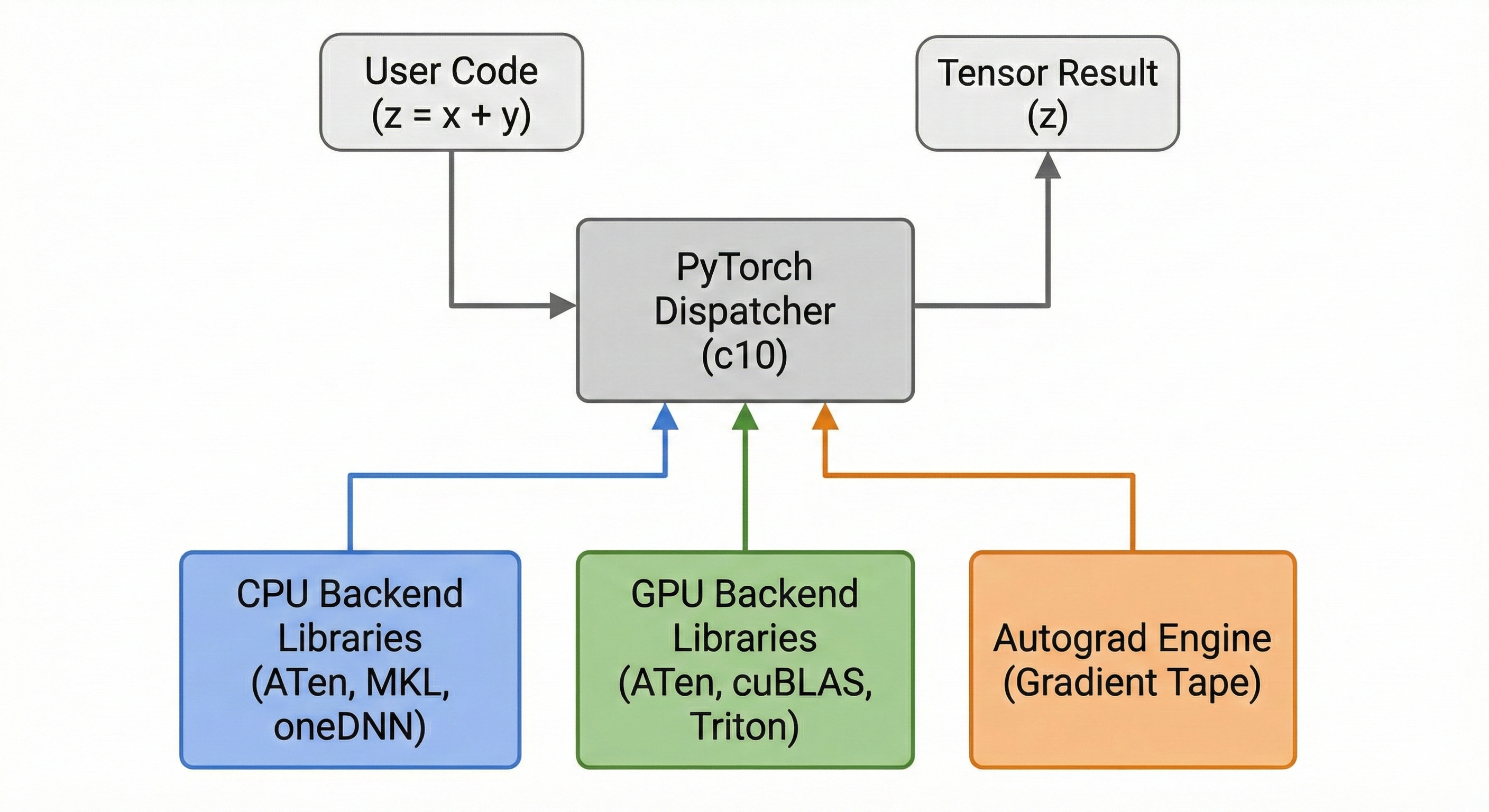
Use Case: PyTorch Dataset#
So, we’ve understood: PyTorch is not easy, and the bottleneck on GPUs is usually data movement—bla bla bla.
But what’s an exciting example to actually understand why this counts? Let’s unwrap an optimization made on a simple task: using a torch.utils.data.DataLoader to feed your model. I see you—you’ve already let Claude code it for you, and it blindly suggested you set pin_memory=True and prefetch_factor=2. Or maybe you didn’t even bother with these optimizations because you figured making your epoch 1% faster wasn’t worth the mental overhead. Fair enough.
But when you’re moving gigabytes of tensor data from a slow SSD to a hungry GPU, that “1%” is actually the difference between your GPU doing actual work and it sitting idle. First of all, we need to understand what these parameters are.
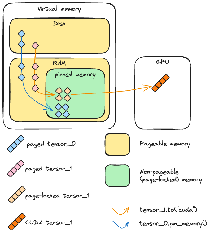
Pin Memory#
RAM is a system organized in pages, which is the main principle of Memory Paging. The Operating System is constantly moving data around to optimize the system, and sometimes data is swapped out from physical memory to the disk.
When the GPU wants data, it can’t just grab it. The CPU first has to move that data into a special, “locked” section of RAM called Pinned (or Page-Locked) Memory. Usually, your data follows this path: Disk -> Pageable RAM -> Pinned RAM -> GPU.
When you tell PyTorch to map the data directly into Pinned RAM to begin with, the GPU grabs it instantly, saving precious milliseconds of CPU overhead. Of course, the downside is that Pinned Memory is “expensive.” You need enough physical RAM to hold these locked buffers, and the time spent “pinning” that memory needs to be lower than the time you’d lose shuffling it around later. If you over-allocate, your OS will start choking on the remaining pageable memory, and you’ll be right back to a slow, messy epoch.
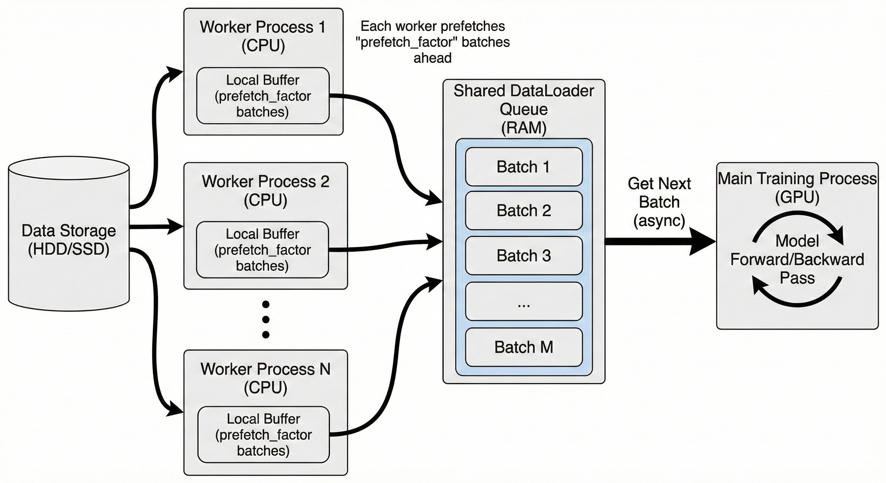
Prefetch Factor#
The Prefetch Factor determines how many batches each worker process should have standing in line, ready to go, before the GPU even asks for them. Usually, your GPU finishes a batch and then waits for the CPU to start loading the next one. If you have num_workers=4 and prefetch_factor=2, your CPU will proactively keep 8 batches sitting in RAM at all times. The moment the GPU finishes Batch N, Batch N+1 is already moving across the PCIe bus.
The Benchmark Paradox#
To address this, let’s look at a benchmark using Optuna with a TPE strategy on a toy model:
search_space = {
    "num_workers": [8, 14],
    "prefetch_factor": [2, 4, 6, 8],
    "pin_memory": [True, False],
    "dataset_type": ["Map", "Iterable"]
}

sampler = optuna.samplers.TPESampler(seed=42)
study = optuna.create_study(direction="maximize", sampler=sampler)

study.enqueue_trial({
    "num_workers": 10,
    "prefetch_factor": 4,
    "pin_memory": False,
    "dataset_type": "Iterable"
})

print("Starting Search...")
study.optimize(objective, n_trials=20)
The results after 20 trials suggested:
Best parameters:
{'num_workers': 10, 'pin_memory': False, 'prefetch_factor': 4, 'dataset_type': 'Iterable'}Best Speed: 34.95 batches/sec
The same configuration with pin_memory = True gives a throughput that is 10–15% lower.
However, trying a real neural network with pin_memory=False gives: Epoch 0: 100%|███| 400/400 [06:24, 1.04it/s]
In contrast, running the same network with pin_memory=True: Epoch 0: 100%|███| 400/400 [06:16, 1.06it/s]
The computation becomes faster with pin_memory=True, despite the initial benchmark suggesting False. These 8 seconds of gain might not seem like much, but at scale, it’s a different story.
The slight speedup during training tells us that computation requires significantly more time than data movement in this specific case. The overhead of organizing pinned memory makes the very first iterations slower, but in the long run, the performance is superior.
Kernels and Benchmark with CPU#
At the end of this gentle introduction to hardware programming, I will offer some simple ways to compute a trivial operation, such as a convolution with a 3x3 symmetric kernel (which is identical to a correlation operation).
There are three versions of the operation presented, using different libraries to highlight their architectural differences:
Numba Kernel: Provides complete control over the workflow. It is the library that best emulates the CUDA programming model, offering a low-level interface with the underlying hardware.
Naive CPU Version: Represents the standard approach for computing operations using plain Python or NumPy on a single processor.
CuPy: A GPU-accelerated library that mirrors the NumPy/SciPy API. In this example, it utilizes an optimized GPU implementation of the
correlate2dfunction.
NUMBA CUDA KERNEL#
@cuda.jit
def conv3x3_kernel(inp, out, k):
    # inp: HxW, out: (H-2)x(W-2), k: 3x3 kernel
    i, j = cuda.grid(2)
    H = inp.shape[0]
    W = inp.shape[1]
    out_H = H - 2
    out_W = W - 2
    if i < out_H and j < out_W:
        s = 0.0
        # apply 3x3 convolution
        for di in range(3):
            for dj in range(3):
                s += k[di, dj] * inp[i+di, j+dj]
        out[i, j] = s
CPU NAIVE#
def conv3x3_cpu(inp, kernel, out):
    """Naive CPU convolution for reference"""
    H, W = inp.shape
    for i in range(H-2):
        for j in range(W-2):
            s = 0.0
            for di in range(3):
                for dj in range(3):
                    s += kernel[di, dj] * inp[i+di, j+dj]
            out[i, j] = s
CUPY IMPLEMENTATION#
def conv3x3_cupy(inp_host, kernel, out, threads=(16,16)):
    """CuPy implementation using scipy-like convolution"""
    inp_d = cp.asarray(inp_host)
    kernel_d = cp.asarray(kernel)
    out = cps.correlate2d(inp_d, kernel_d, mode='valid')
We can run a benchmark with these functions, paying close attention to the speedup relative to the CPU version, as well as the time allocated to computation versus data movement.
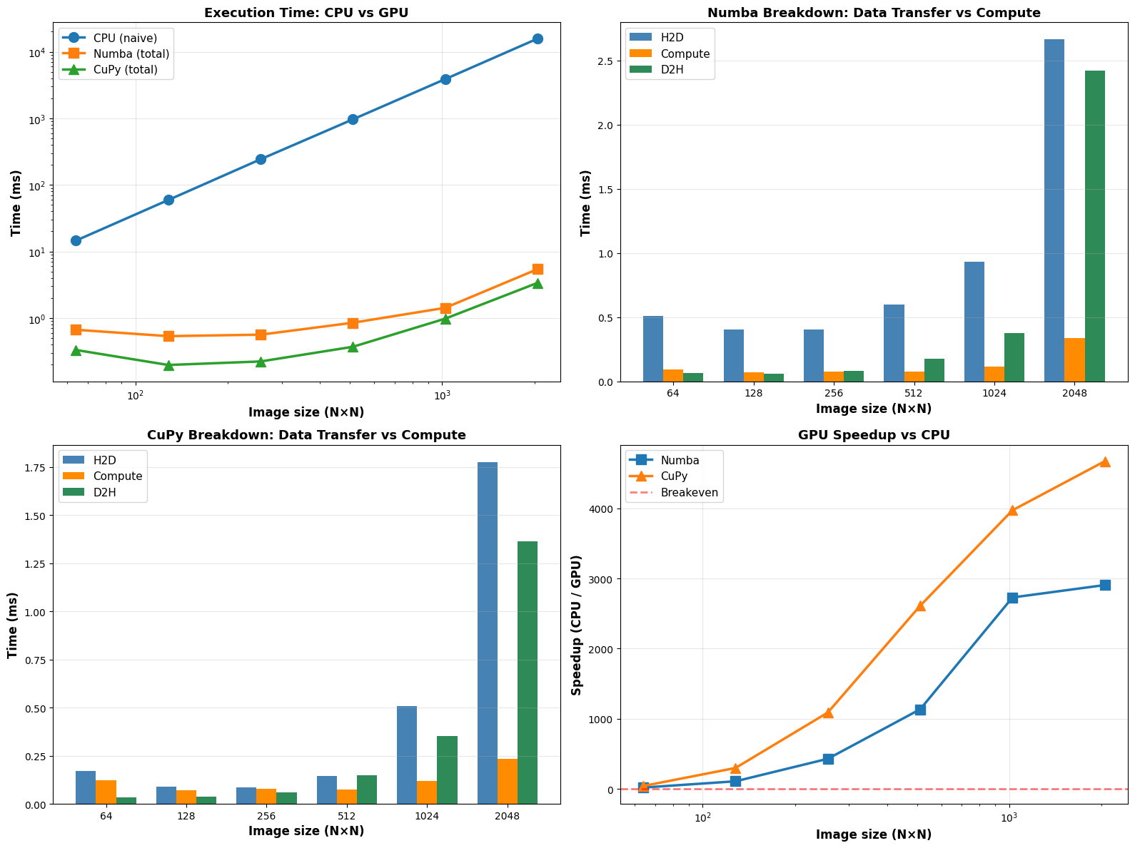
Based on the benchmark results, there are several key takeaways regarding hardware acceleration and the “cost” of moving data to the GPU.
As illustrated, the Execution Time and Speedup charts tell a clear story: while the CPU’s execution time increases significantly as the image size grows, the GPU versions remain relatively flat until reaching much larger workloads. At the largest test size ($2048 \times 2048$), CuPy achieves a massive speedup of over 4,500x compared to the naive CPU implementation. Numba is slightly slower but still delivers a nearly 3,000x speedup. This performance gap is expected, as our custom Numba kernel was not optimized to the same degree as the built-in CuPy functions.
The most insightful data comes from the Breakdown graphs (H2D: Host-to-Device; D2H: Device-to-Host). For both Numba and CuPy, the actual Compute time (the orange bars) is almost negligible compared to the time spent moving data. H2D (Blue) is the primary bottleneck. This confirms that for small images (e.g., $64 \times 64$), the GPU may offer little to no benefit because the time spent “sending the image to the card” outweighs the raw processing speed.
Key Takeaways:#
Scale Matters: GPU acceleration is a “high-overhead” strategy. It is only advantageous when the computational complexity is high enough to justify the data transfer penalty.
Library Efficiency: CuPy performs better here likely due to its highly optimized underlying C++/CUDA kernels, whereas a custom Numba kernel requires careful manual tuning to reach peak performance.
Minimize Movement: To maximize efficiency in a real-world pipeline, data should remain on the GPU between operations to avoid repeating these expensive H2D and D2H transfers.