Introduction and Motivation#

Bridging the gap between how cameras capture the two-dimensional world and how computers understand three-dimensional space has long been a holy grail of computer vision. While traditional computational methods are truly useful, they have historically struggled with reflective surfaces, transparent objects, and untextured walls, or require an enormous, dense matrix of cameras and massive amounts of storage.

Nonetheless, traditional methods remain the most widely used in many industrial tasks that demand real-world physical measurements with millimeter accuracy. However, when photorealistic results are needed or highly complex, difficult objects are being scanned, it makes sense to turn to these techniques.

During this dissertation, we will explore newer deep learning methods with a focus on edge/real-time constraints. We will also examine how these methods address common challenges.

Glossary#

Plenoptic Function#

Given a scene, the plenoptic function is a full description of all the light rays that travel across the space. The plenoptic function tells us the light intensity of a light ray passing through the three-dimensional (3D) point  from the direction given by the angles , with wavelength $\lambda$, at time $t$. For the sake of simplicity we will ignore time and we will only use three color channels (RGB) instead of the continuous wavelength. We can represent the plenoptic function with the parametric form where the parameters  have to be adapted to represent each scene.

$$L(X, Y, Z, \psi, \phi)$$

It now asks:

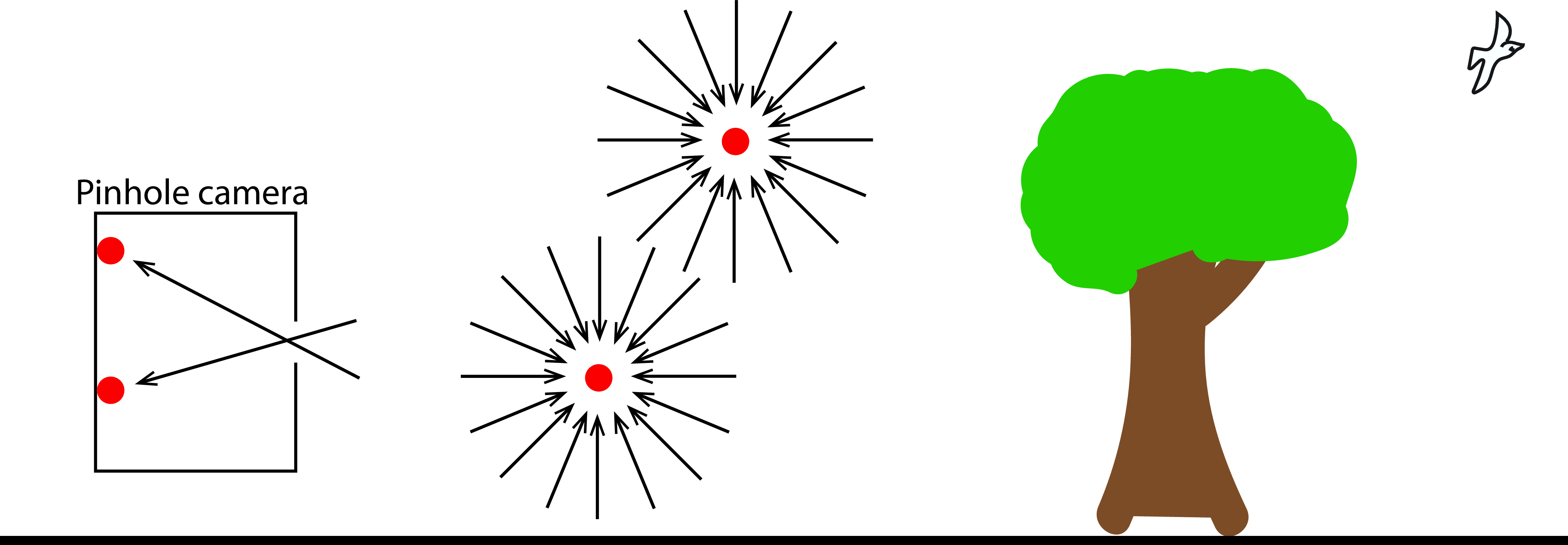
It asks the question: “If I am standing at a specific point in 3D space $(x,y,z)$, and I look in a specific angular direction $(\theta,\phi)$, what color do I see?”

If we had access to the plenoptic function of a scene, we would be able to render images from all possible viewpoints within that scene. The following methods aim to approximate and query the plenoptical function of a specific scene.

Radiance Field#

A Radiance Field is a formal function describing how light flows through a D-dimensional space.

Neural Field#

A neural field, is a vector field that is fully or partially parametrized by a neural network. Differently from traditional machine learning algorithms, neural fields do not work with discrete data, but map continuous inputs to continuous outputs. This makes neural fields not only discretization independent, but also easily differentiable.

Implicit Radiance Field#

If you want to know what color a point in the room is, you can’t just look it up. You have to feed the coordinate into a massive equation (the MLP) and let it compute the answer. Because the network smoothly interpolates between points, it is highly data-efficient and excellent at capturing fine geometry, but calculating thousands of rays per second is computationally taxing.

Explicit Radiance Field#

Think of this like a physical 3D grid or a cloud of colored particles. The space is broken down into structured elements, such as a voxel grid (Plenoxels) or millions of tiny 3D ellipsoids (3D Gaussian Splatting). To render an image, the computer simply projects these physical shapes onto the screen (rasterization). It skips the heavy neural network math entirely, unlocking blistering real-time speeds at the cost of high storage usage.

Differentiable Rendering#

A rendering pipeline where every step is mathematically differentiable. This allows the system to use gradient descent to minimize the error between a rendered image and a real ground-truth photograph.

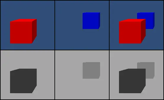
To provide a counter-example, the most classic case is Traditional Rasterization with a Z-Buffer. Imagine you have a red square on a blue background, and you want to optimize its position so that it matches a target image. When a object is rendered, the depth of a generated pixel(z coordinate) is stored in the depth buffer. If another object must be painted in the same pixel, the depth of the new pixel is compared with the stored depth, In a traditional renderer, a this is determined by a conditional check:

if (object_is_present_at_pixel) then color = RED else color = BLUE

Mathematically, this is a step function that is obviously not differentiable.

# Neural Radiance Fields

In contrast to explicit representations, Neural Radiance Fields (NeRF) represent a scene implicitly through a continuous function $F_\Theta$, typically parameterized by a multilayer perceptron (MLP).

Coordinate Mapping#

The core mathematical formulation maps a 5D input, composed by a 3D spatial location $\mathbf{x} = (x, y, z)$ and a 2D viewing direction $\mathbf{d} = (\theta, \phi)$, to a volume density $\sigma$ and a view-dependent RGB color $\mathbf{c} = (r, g, b)$, so ending in an output ($\sigma$, $\mathbf{c}$).

Continuous Volume Rendering#

To render a single pixel, NeRF employs volume rendering integrals; for a camera ray $\mathbf{r}(t) = \mathbf{o} + t\mathbf{d}$ with near and far bounds $t_n$ and $t_f$, the expected color $C(\mathbf{r})$ is calculated as:

$$C(\mathbf{r}) = \int_{t_n}^{t_f} T(t) \sigma(\mathbf{r}(t)) \mathbf{c}(\mathbf{r}(t), \mathbf{d}) dt$$

where $T(t)$ represents the accumulated transmittance along the ray from $t_n$ to $t$:

$$T(t) = \exp\left( -\int_{t_n}^{t} \sigma(\mathbf{r}(s)) ds \right)$$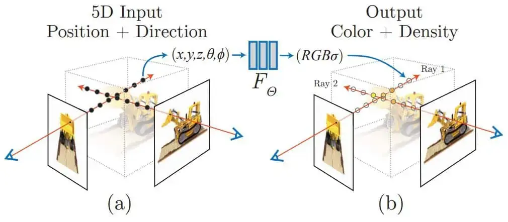

Numerical Integration via Quadrature#

In practice, this continuous integral is estimated using quadrature by sampling $N$ points along the ray.

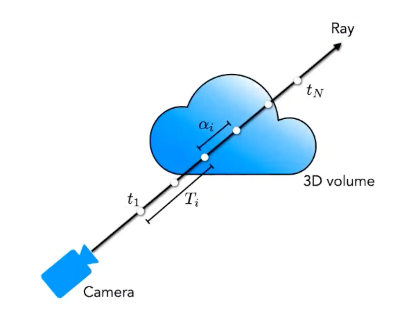
The discretized rendering equation becomes:

$$\hat{C}(\mathbf{r}) = \sum_{i=1}^{N} T_i (1 - \exp(-\sigma_i \delta_i)) \mathbf{c}_i$$

where $\delta_i = t_{i+1} - t_i$ is the distance between adjacent samples, and $T_i = \exp(-\sum_{j=1}^{i-1} \sigma_j \delta_j)$. This function is trivially differentiable and reduces to traditional alpha-compositing with alpha values $\alpha_i = 1 - \exp(-\sigma_i \delta_i)$.

To capture high-frequency details, the input coordinates are projected into a higher-dimensional space using positional encoding $\gamma(p) = (\sin(2^0\pi p), \cos(2^0\pi p), \dots, \sin(2^{L-1}\pi p), \cos(2^{L-1}\pi p))$, allowing the MLP to overcome the spectral bias of neural networks toward low-frequency functions.

The model is optimized by minimizing the total squared error between the observed pixel colors and the rendered values:

$$\mathcal{L} = \sum_{\mathbf{r} \in \mathcal{R}} \| \hat{C}(\mathbf{r}) - C_{gt}(\mathbf{r}) \|_2^2$$

Hierarchical sampling#

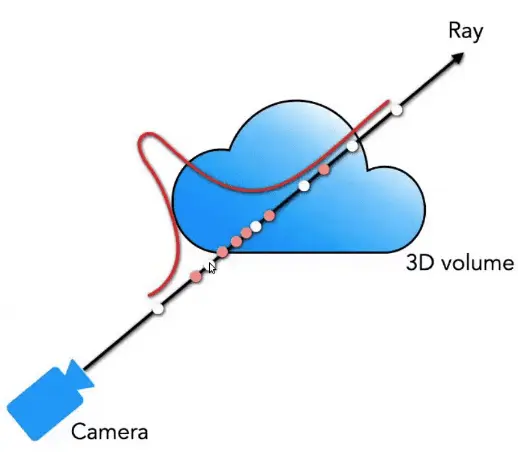
Hierarchical Volume Sampling is a strategy used to solve the efficiency problem of sampling points along a ray.

If you sample points uniformly along a ray, most of those points will be in empty space (where density ) or behind occluded surfaces, contributing nothing to the final image. Hierarchical sampling ensures that the computer’s “effort” is focused on the parts of the ray that actually contain the object.

The process involves two simultaneous networks: the Coarse Network and the Fine Network.

Coarse Stage#

First, the algorithm samples a small number of points $N_c$ (64 in the original paper) at uniform intervals along the ray. It passes these points through the “Coarse” MLP to get an initial estimate of the density along the ray.

Using these densities, we calculate a weight for each sampled point, which tells us how much that point contributes to the final pixel color.

These weights are normalized to create a Probability Density Function (PDF) along the ray.

This PDF essentially acts as a map, telling the system: “The object surface is likely located in these specific regions where the weights are high.”

The Fine Stage#

Next, a second set of  points $N_f$ (128 in the original paper) is sampled using Inverse Transform Sampling based on the PDF created in the previous step. This forces the algorithm to place more samples in regions with high density (the object’s surface) and fewer samples in empty space.

The “Fine” MLP is then evaluated using the total set of  samples.

Because the samples are now concentrated around the actual geometry of the scene, the fine network can capture much more detail, sharper edges, and more accurate textures than the coarse network alone.

Architectural & Parameter Breakdown#

To determine the memory footprint, we first calculate the exact number of trainable parameters.

This model assumes a standard MLP architecture without additional input expansion or architectural shortcuts.

Layer Description	Calculation	Parameters
Layer 1 (Input 3 → 256)	$(3 \times 256) + 256$	1,024
Layers 2–8 (7 layers, 256 → 256)	$7 \times [(256 \times 256) + 256]$	460,544
Density ($\sigma$) Output (256 → 1)	$(256 \times 1) + 1$	257
Color Net Input (256 + 3 view dir = 259)	—	—
Additional Layer (259 → 128)	$(259 \times 128) + 128$	33,280
RGB Output (128 → 3)	$(128 \times 3) + 3$	387
TOTAL		~495,492

The classic implementation version includes also high-frequency positional encoding ($L=10$ for coordinates, $L=4$ for viewing directions) and a skip connection at Layer 5. This lead to an Input Expansion from 3D coordinates to 60 dimensions, while the view direction expands to 24 dimensions. So at the end the number of trainable parameters are:

Total Parameter Count For Vanilla NeRF: ~528,132

While the model itself is lightweight, the memory dynamics shift drastically once training begins.

---

Static Memory: Model & Optimizer#

Because the network is relatively small (~0.5M parameters) compared with modern architectures, the physical footprint on disk or in VRAM is negligible by modern standards.

Component	Calculation	Memory Usage
Model Weights (FP32)	$528,132 \text{ params} \times 4 \text{ bytes}$	~2.1 MB
Optimizer States (Adam)	$528,132 \text{ params} \times 12 \text{ bytes}$	~6.3 MB
Total Static Footprint		~8.4 MB
The true architectural challenge is activation memory.
Because NeRF relies on volumetric rendering via stochastic ray sampling, the GPU must cache activations for every sampled point to facilitate backpropagation.

• Ray Samples: 4,096 rays/batch $\times$ 64 samples/ray = 262,144 points
• Requirement: Storing 8 layers of activations for every one of those 262,144 points.

VRAM Utilization Breakdown#

Configuration	Point Samples per Batch	Estimated VRAM Usage
Coarse Network Only	262,144	2 – 3 GB
Coarse + Fine Networks	~786,432	6 – 8 GB

---

Even with modern flagship hardware like the RTX 4090 or A100, the “vanilla” NeRF architecture remains surprisingly demanding. The bottleneck is not the size of the model, but the sheer volume of queries required to integrate radiance along a single ray.

Performance Metrics#

For a standard 800x800 resolution frame with 192 samples per ray, the MLP must perform roughly 122 million inferences to render a single view.

Metric	Performance Detail
Training Duration	1 – 3 hours (for 200k–300k iterations)
Inference (Rendering)	1 – 5 seconds per frame
Primary Bottleneck	Memory bandwidth & Batch overhead

---

The “Small Model” Bottleneck#

It is counter-intuitive that a 0.5M parameter model takes hours to train. However, the hardware faces two specific limitations:

1. Memory Bandwidth vs. Compute: Because the MLP is so small, the GPU’s massive core count often sits idle while waiting for the next set of ray coordinates to be fetched from memory. The workload is “compute-bound” only for the actual matrix multiplication, but “memory-bound” for the bulk of the rendering pipeline.
2. Kernel Launch Overhead: Processing hundreds of thousands of tiny samples involves significant overhead in launching CUDA kernels. Because the batch sizes are small relative to the GPU’s massive throughput, the GPU struggles to saturate its arithmetic logic units (ALUs).

---

Scaling Perspective#

While an RTX 4090 or A100 can comfortably handle this in a few hours, the process remains computationally expensive due to the nature of volumetric rendering:

• Iteration Scaling: 300,000 iterations $\times$ 262,144 points per batch = ~78 Billion neural network evaluations per training session.
• Real-time vs. NeRF: To achieve “real-time” rendering (30+ FPS), you would need to process 19 million rays per second. At 192 samples per ray, this equates to ~3.6 billion MLP queries per second, which remains far beyond the capabilities of a raw vanilla MLP without architectural acceleration.

Methods for fast adaptation#

Neural Radiance Caching#

In a real-time path tracing environment, you only have a budget of a few milliseconds to query millions of points. General frameworks are designed for large-batch throughput, not the ultra-low latency required for per-frame radiance estimation.

As stated in the original paper:

Our system is designed according to the following principles:

• Dynamic content: To handle fully interactive content, the system must support arbitrary dynamics of the camera, lighting, geometry, and materials. We strive for a solution that does not require precomputation.
• Robustness: Case-specific handling eventually leads to complex, brittle systems. Hence, the cache should be agnostic of materials and scene geometry… additional attributes may be provided to the system to improve its rendering quality.
• Predictable performance and resource consumption: Fluctuations in workload and memory usage lead to unstable framerates. We seek a solution with stable runtime overhead and memory footprint, both of which should be independent of scene complexity.

Instead, we build on the simple but powerful realization that the generalization challenge can be completely sidestepped by fast adaptation.

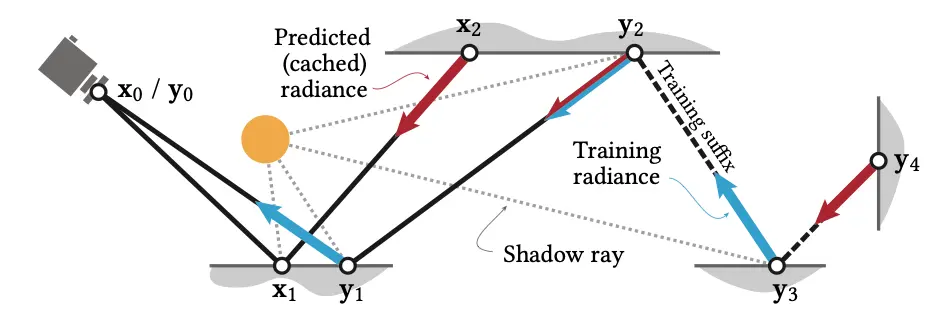
The NRC kernel acts as a “short-circuit” for path tracing. Instead of tracing a ray through 10 bounces (which is slow), the system traces 2 bounces and then queries the ad-hoc MLP kernel, that acts as a cache, to “predict” the remaining light.

This hybrid approach combines:

1. Ray Tracing: For high-frequency, near-field details.
2. Neural Caching (via fused kernels): For complex, multi-bounce global illumination that would otherwise be too noisy or slow to compute in real-time.

Kernel Launch and Memory Overhead#

In a standard MLP implementation, each layer (Linear, ReLU, etc.) involves a separate CUDA kernel launch. For a small “bottleneck” MLP like those used in NRC or Instant-NGP:

1. Launch Overhead: The time spent by the CPU telling the GPU to start a kernel becomes a significant percentage of the total execution time.
2. VRAM Round-trips: Each layer reads its input from Global Memory (VRAM) and writes its output back to VRAM. Since small MLPs are “memory-bound,” the GPU spends more time moving data than actually performing the math.

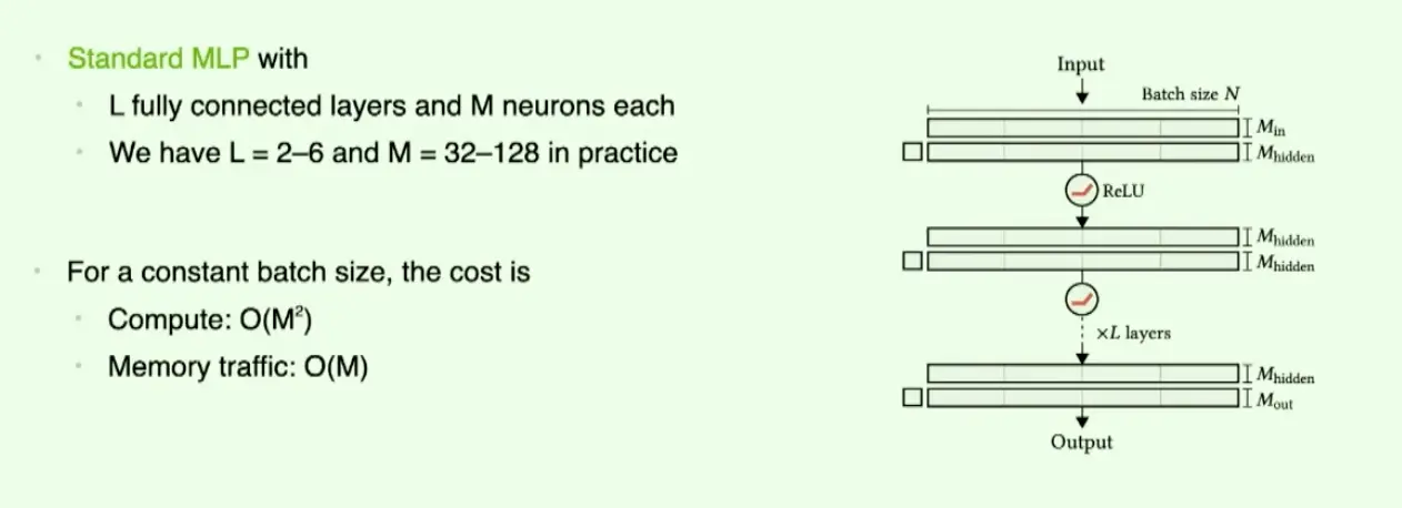
Usually, with that compute it can make sense to focus on computation but on modern GPUs on small numbers of neurons the memory traffic impacts the performances a lot, so the idea behind was pretty simple, we can allocate wisely the blocks for the matrix multiplication in order to avoid loading from RAM each time we have to perform an activation.

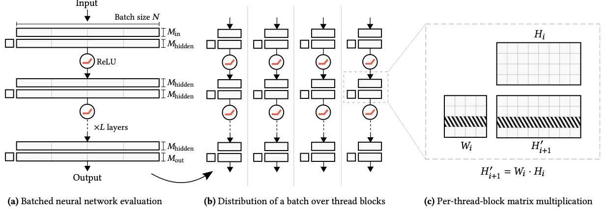
That’s what happens here, basically each parallel stream is loaded only once from RAM, for this reason it makes the computational overhead of getting the data from Global Memory significantly lower, as the GPU avoids redundant read/write cycles and instead performs all operations within high-speed registers or Shared Memory, effectively shifting the bottleneck from memory bandwidth to the raw compute throughput of the streaming multiprocessors.

Instant-NGP#

The “vanilla” NeRF architecture suffers from a performance bottleneck where it takes hours to train due to the massive number of neural network evaluations (~78 billion per session).

Instant-NGP (Instant Neural Graphics Primitives), solves this by shifting the computational burden from the neural network to a specialized data structure. The core concept is Multi-Resolution Hash Encoding.

Instead of forcing a single MLP to learn and “memorize” the entire 3D scene (which is what makes the MLP large and slow), Instant-NGP stores the scene information in a set of feature vectors organized in a grid. The MLP becomes a “tiny” decoder that only translates these features.

Storing a high-resolution 3D grid would require a massive amount of VRAM. Instant-NGP solves this by:

• Mapping the vertices of these grids to a fixed-size hash table.
• Even if two different spatial points “collide” (map to the same hash entry), the neural network learns to disambiguate them during training without further effort.
• This allows for a very high-resolution representation with a very small memory footprint.

Because the hash table does most of the “heavy lifting” by providing rich spatial features, the MLP used in Instant-NGP is extremely small (often only 2 or 3 layers deep).

Multi-Resolution Hashing#

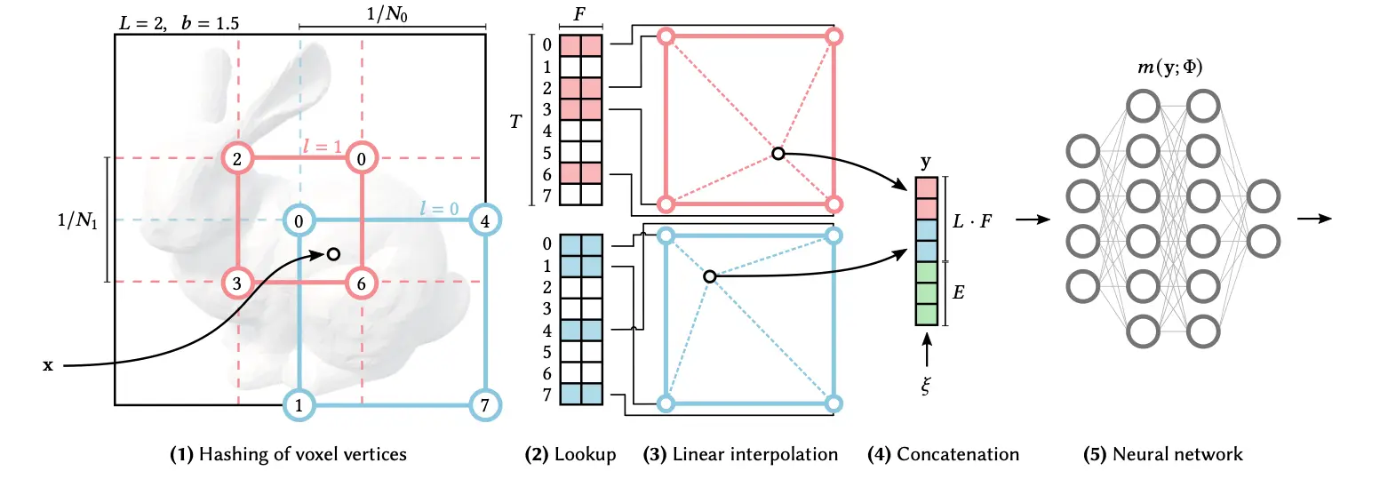
Instant-NGP introduces Multi-Resolution Hash Encoding, which stores scene features in a hierarchy of $L$ grid levels. For an input 3D coordinate $\mathbf{x}$, the system identifies the surrounding voxels at each resolution level $l \in [0, L-1]$. The resolution $N_l$ of each level typically follows a geometric progression between a minimum resolution $N_{min}$ and a maximum resolution $N_{max}$:

$$N_l = \lfloor N_{min} \cdot b^l \rfloor, \quad b = \exp\left( \frac{\ln N_{max} - \ln N_{min}}{L-1} \right)$$

At each level $l$, the corners of the voxel grid $\mathbf{v}$ are mapped to a feature vector in a hash table of fixed size $T$ using a spatial hash function:

$$h(\mathbf{v}) = \left( \bigoplus_{i=1}^d v_i \cdot \pi_i \right) \pmod T$$

where $\oplus$ denotes the bitwise XOR operation, $d=3$ for 3D space, and $\pi_i$ are large unique prime numbers (e.g., $\pi_1 = 1, \pi_2 = 2,654,435,761, \pi_3 = 805,459,861$). This hashing allows the system to represent a high-resolution sparse volume without the $O(N^3)$ memory cost of a dense grid. The features at each level are retrieved via trilinear interpolation of the hashed vertex values:

$$f_l(\mathbf{x}; \Phi_l) = \text{interp}(\mathbf{x}, \{ \Phi_l[h(\mathbf{v})] \}_{\mathbf{v} \in \text{cell}(\mathbf{x}, l)})$$

The final encoded representation $\gamma(\mathbf{x})$ is the concatenation of the interpolated features from all $L$ levels, augmented with auxiliary inputs such as viewing direction $\mathbf{d}$ (often encoded via Spherical Harmonics):

$$y = [f_0(\mathbf{x}), f_1(\mathbf{x}), \dots, f_{L-1}(\mathbf{x}), \text{enc}(\mathbf{d})]$$

This high-dimensional feature vector $y$ is then processed by a very small “bottleneck” MLP. By shifting the complexity from the neural weights to this indexed data structure, Instant-NGP reduces the number of floating-point operations per ray sample by several orders of magnitude, enabling convergence in seconds rather than days.

Based on the previous calculation of 262,144 points per batch, we can see why Instant-NGP offers a massive performance leap over the “vanilla” architecture.

The performance improvement stems from how the system handles those 262,144 neural network evaluations per batch:

Reduction in MLP Workload#

In Vanilla NeRF, every one of those 262,144 points must pass through a deep MLP (typically 8 layers of 256 neurons). This requires massive matrix multiplications for every single sample point. Instant-NGP replaces the deep MLP with a Multi-Resolution Hash Table. Most of the scene’s complexity is “stored” in the hash grid, allowing the MLP to be “tiny” (often only 2 layers of 64 neurons). The computational cost per point drops from thousands of floating-point operations to just a few dozen.

$O(1)$ Feature Retrieval vs. Learned Mapping#

• Vanilla NeRF uses the MLP to “calculate” the density and color from scratch using Positional Encoding.
• Instant-NGP uses trilinear interpolation to “look up” the features. Since the hash table lookup and trilinear interpolation are $O(1)$ operations, the system can process the 262,144 points significantly faster than a neural network can compute them.

Performance Comparison Table#

Metric	Vanilla NeRF	Instant-NGP
MLP Depth	8+ Layers	2-3 Layers
Feature Extraction	Trigonometric Calculation (Positional Encoding), not GPU-friendly	Hash Table Lookup + Interpolation
Operations per Point	High (Heavy Matrix Multiply)	Low (Simple Arithmetic)
Training Time	1 – 2 Days	5 Seconds – 2 Minutes
Total Iterations	~300,000	~10,000 - 30,000

Convergence Efficiency#

Because the hash grid provides a more explicit spatial structure than a “black box” MLP, the optimizer finds the correct geometry much faster. While your implementation details suggest 100k–300k iterations for vanilla NeRF, Instant-NGP often achieves better visual quality in less than 10k iterations, making each of those 262,144-point batches count for more progress toward the final image.

The hash table size is a critical hyperparameter that balances the trade-off between reconstruction quality and memory consumption. As you noted from the batch calculation, a single training step processes 262,144 points; the relationship between these points, the grid vertices, and the hash table size $T$ is what defines the efficiency of the system.

Hash Table Dimensions#

The “size” of the hash encoding is defined by three main parameters:

• $L$ (Number of Levels): Typically 16 levels.
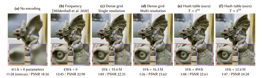
• $T$ (Table Size/Capacity): The number of entries in the hash table for each level, usually ranging from $2^{14}$ to $2^{24}$ (524,288 entries is a common default, i.e., $2^{19}$).
• $F$ (Feature Dimension): The number of learnable values per entry, typically 2.

The total number of trainable parameters in the hash grid is therefore $L \times T \times F$.

When Grid Vertices Exceed Table Size ($V > T$)#

At coarse resolutions, the number of grid vertices $V = (N+1)^3$ is smaller than the table size $T$. In this case, the mapping is 1:1, meaning every spatial vertex has its own unique feature vector.

However, at finer resolutions (high $l$), the grid becomes extremely dense. For example, at a resolution of $N=2048$, there are over 8 billion potential vertices ($2048^3$). Since $T$ is much smaller (e.g., $2^{19} \approx 5 \times 10^5$), multiple distinct spatial vertices will inevitably map to the same index in the hash table. This is known as a hash collision.

Impact of Collisions on the 262,144 Sample Points#

When you process a batch of 262,144 points, many of these points will fall into different grid cells that technically “collide” in the hash table. The system handles this through two mechanisms:

• The Multi-Resolution Advantage: Because the hash tables are independent across $L$ levels, it is highly unlikely that two spatial points will collide at every resolution level simultaneously. While they might collide at a fine resolution, their features at a coarser or medium resolution will remain distinct, allowing the MLP to differentiate them.
• Gradient Averaging: During the optimization of a batch, if two points (one in empty space, one on a solid surface) map to the same hash entry, the point on the surface will provide a much stronger gradient to the loss function. The MLP effectively learns to “ignore” the noise caused by collisions in empty space and prioritizes the feature values that contribute to the visible geometry of the scene.

Summary Table: Resolution vs. Hashing#

Grid Level	Resolution ($N_l$)	Vertices ($V$)	Mapping Type	Memory Usage
Coarse	Low (e.g., 16)	$17^3 = 4,913$	Direct (1:1)	Low
Fine	High (e.g., 2048)	$2049^3 \approx 8.6B$	Hashed (Many:1)	Capped at $T$

If the hash table size $T$ is significantly lower than the number of points sampled in a batch (e.g., $T=16k$ while samples = $262k$), the “collisions” become too frequent, and the MLP may struggle to resolve the ambiguity, leading to “ghosting” artifacts or a loss of fine detail in the reconstruction.

GNeRFs#

The original Neural Radiance Field (NeRF) paper had a massive bottleneck: per-scene optimization. To render a novel view, you had to train a neural network from scratch for hours on dozens of images of that specific scene.

Generalizable NeRFs solve this by learning a prior across multiple scenes during training. Instead of memorizing a single scene, the network learns how to map 2D image features from a few source views directly into a 3D radiance field. This allows for zero-shot or few-shot novel view synthesis in seconds or minutes.

pixelNeRF#

pixelNeRF is an architecture designed to overcome one of the primary limitations of vanilla NeRF: the lack of generalization. While standard NeRFs require hours of training for a single specific scene, pixelNeRF allows the model to predict a radiance field from just one or a few input images by learning a prior across different scenes.

Core Mechanism: Image Conditioning#

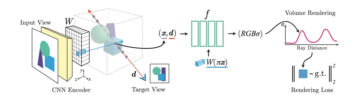
The fundamental shift in pixelNeRF is that the MLP is no longer just a function of coordinates, but is conditioned on local image features.

• Feature Extraction: Unlike the “vanilla” approach, pixelNeRF uses a Convolutional Neural Network (CNN), such as a ResNet, to extract a feature map from the input images.
• Spatial Projection: For any 3D query point $\mathbf{x}$ along a ray, the model projects that point back onto the 2D image plane of the input views.
• Local Features: The model extracts the local feature vector from the feature map at that projected 2D location (using bilinear interpolation).
• Conditioned MLP: The MLP then takes both the 3D coordinate and the extracted local feature to predict the volume density $\sigma$ and color $\mathbf{c}$.

Key Advantages#

• Generalization: It can be trained on a large dataset of objects (like ShapeNet) and then used to reconstruct a completely new, unseen object without needing to re-train the network weights.
• Few-Shot Reconstruction: It works with as little as a single input image (1-view), whereas vanilla NeRF would fail to resolve any geometry.
• Coordinate Frame: The radiance field is defined in the camera’s coordinate system rather than a global world system, which simplifies the learning of geometric priors.

Comparison with Vanilla NeRF#

Feature	Vanilla NeRF	pixelNeRF
Input	Many views of 1 scene	1 or more views + learned priors
Training	Per-scene optimization	Pre-trained on a dataset
Latency	Hours to optimize	Instant (feed-forward inference)
Geometry	Learned from scratch	Derived from image features

## MVSNeRF

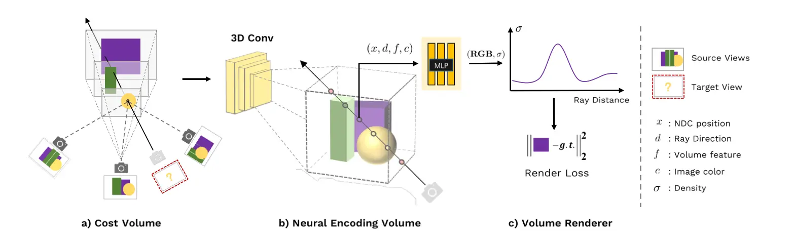
MVSNeRF (Multi-View Stereo Neural Radiance Fields) is a generalizable neural rendering approach that, like pixelNeRF, aims to reconstruct new scenes without the lengthy per-scene optimization required by vanilla NeRF.

The key innovation of MVSNeRF is its use of a 3D Cost Volume derived from traditional Multi-View Stereo (MVS) techniques to provide the neural network with a geometric “roadmap.”

Cost Volume Construction#

Instead of just projecting 3D points onto 2D images, MVSNeRF builds a Plane Sweep Volume:

• Feature Extraction: It uses a 2D CNN to extract feature maps from a small set (usually 3) of nearby input images.
• Homography Warping: It warps these features into a reference camera’s frustum at different depth planes.
• Cost Volume: By measuring the variance (consistency) between these warped features across the depth planes, it creates a 3D volume where high consistency likely indicates the presence of a surface.

Hybrid Representation#

MVSNeRF is a hybrid between Explicit and Implicit representations:

• Explicit Component: A 3D CNN processes the Cost Volume to produce a “Neural Encoding Volume.” This volume stores local geometric and appearance information in a structured grid.
• Implicit Component: A lightweight MLP then queries this encoded volume. For any 3D point $\mathbf{x}$, the MLP interpolates the neighboring features from the volume to predict volume density $\sigma$ and RGB color $\mathbf{c}$.

Computational Efficiency and Memory#

MVSNeRF is designed to optimize the data flow:

• Reduced MLP Load: Because the 3D Cost Volume provides a dense geometric “roadmap,” the MLP does not need to learn the scene from scratch. This allows for a much shallower and narrower MLP compared to vanilla NeRF, drastically reducing the total number of floating-point operations (FLOPs) required to render a pixel.
• Inference Speed: While the 3D CNN used to process the cost volume is computationally heavy during the initial pass, it only needs to be computed once for a set of reference images. Subsequent novel view synthesis is fast because it involves simple trilinear interpolation of the “Neural Encoding Volume,” shifting the bottleneck from heavy neural computation to efficient spatial lookups.

Comparison with Vanilla NeRF#

Feature	Vanilla NeRF	MVSNeRF
Geometry Source	Learned via optimization	Derived via Plane Sweep (MVS)
Generalization	None (1 model per scene)	High (Pre-trained on datasets)
Input Requirement	50–100+ images	~3 sparse images
Rendering Speed	Slow (Heavy MLP)	Fast (Voxel-based interpolation + light MLP)
Storage	Small (MLP weights)	Large (Cost Volume / Voxel grid)

# Gaussian Splatting

Moving from implicit functions to explicit representations, 3D Gaussian Splatting represents the scene using a collection of millions of learnable 3D Gaussians.

Initialization#

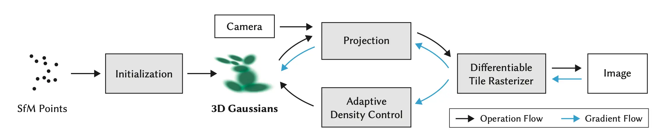
Unlike “vanilla” NeRFs, which typically initialize with random neural network weights, 3DGS relies on a geometric “head start” provided by Structure from Motion (SfM). A tool like COLMAP is usually used to process the input images performing:

1. Camera Calibration: It determines the precise position and orientation (intrinsics and extrinsics) of the camera for every photo.
2. Sparse Point Cloud Generation: It identifies matching features across different images to triangulate points in 3D space.

Method#

Each Gaussian is defined by a center position $\mathbf{\mu} \in \mathbb{R}^3$, an opacity $\alpha \in [0, 1]$, a color $\mathbf{c} \in \mathbb{R}^3$, and a 3D covariance matrix $\Sigma$ that describes its shape and orientation.

To ensure that $\Sigma$ remains positive semi-definite during optimization, it is factorized into a scaling matrix $S$ and a rotation matrix $R$ (represented by a quaternion):

$$\Sigma = RSS^T R^T$$

The spatial influence of a Gaussian at a point $\mathbf{x}$ is given by the probability density function:

$$g(\mathbf{x}) = \exp\left(-\frac{1}{2}(\mathbf{x}-\mathbf{\mu})^T \Sigma^{-1} (\mathbf{x}-\mathbf{\mu})\right)$$

To render these primitives onto a 2D image plane, the 3D Gaussians are projected into 2D “splats.” Given a viewing transformation $W$ and the Jacobian $J$ of the affine approximation of the projective transformation, the 2D covariance matrix $\Sigma'$ in image coordinates is calculated as:

$$\Sigma' = J W \Sigma W^T J^T$$

The final color $C$ of a pixel is determined by sorting the Gaussians by depth and performing alpha-blending, which is mathematically equivalent to the volumetric rendering equation but applied to discrete primitives. For a set of $N$ ordered Gaussians overlapping a pixel, the color is accumulated as:

$$C = \sum_{i=1}^{N} \mathbf{c}_i \alpha'_i \prod_{j=1}^{i-1} (1 - \alpha'_j)$$

where $\mathbf{c}_i$ is the color of the $i$-th Gaussian (typically represented using Spherical Harmonics to capture view-dependency) and $\alpha'_i$ is the effective opacity, calculated by multiplying the base opacity $\alpha_i$ by the Gaussian’s 2D spatial influence $g'(\mathbf{x})$. This explicit formulation allows to bypass the expensive MLP evaluations required by NeRF, enabling real-time rendering speeds through highly optimized tile-based rasterization.

Training#

The training procedure employs Stochastic Gradient Descent (SGD) to optimize the explicit Gaussian parameters. Unlike NeRF, which optimizes the weight matrices of a neural network, 3DGS optimizes the geometric and appearance properties of the primitives directly.

The training cycle consists of the following steps:

• Differentiable Rasterization: The current set of Gaussians is projected onto the image plane to generate a synthetic view using the tile-based rasterization pipeline.
• Loss Computation: The system calculates the error (typically a combination of $L_1$ and SSIM loss) between the rasterized image and the ground truth photograph.
• Parameter Adjustment: The loss is backpropagated to update the position $\mathbf{\mu}$, covariance $\Sigma$, color $\mathbf{c}$, and opacity $\alpha$ of each Gaussian.
• Adaptive Density Control: Periodically, the system refines the number and distribution of Gaussians to better represent the scene:
  • Splitting and Cloning: If the gradient for a specific Gaussian is large (indicating high reconstruction error), the system clones it if it is small, or splits it into two smaller Gaussians if it is large.
  • Pruning: Any Gaussian whose opacity $\alpha$ drops below a defined threshold or that grows to an unnaturally large size is removed.

Radix Sort#

To ensure correct alpha blending (the “Over” operator), 3D Gaussians must be rendered in a specific order. This requires a highly efficient sorting mechanism to handle millions of primitives in real-time.

Radix sort is a non-comparative sorting algorithm that avoids the $O(n \log n)$ bottleneck of traditional comparison-based sorts like QuickSort. Instead of comparing pairs of values, it processes the individual bits of the depth values (the keys).

The process involves:

• Key Generation: The 3D depth of each Gaussian center is projected and converted into a 32-bit or 64-bit integer key.
• Digit Grouping: The algorithm iterates through the bits of these keys from the least significant to the most significant (or vice versa), grouping the Gaussians into “buckets” based on those bits.
• Parallel Prefix Sum (Scan): On the GPU, the algorithm uses a “parallel scan” to calculate the offsets for each bucket, allowing every thread to know exactly where to move its assigned Gaussian in the final sorted array.
• Stable Permutation: Because it is a stable sort, it maintains the relative order of Gaussians that have identical or nearly identical depth values, preventing flickering artifacts.

In the context of 3D Gaussian Splatting, Radix sort is preferred over other algorithms for several technical reasons:

• Linear Time Complexity: For a fixed number of bits (like 32-bit depth values), Radix sort operates in $O(n)$ time.
• Hardware Synergy: The algorithm is perfectly suited for the GPU’s SIMT (Single Instruction, Multiple Threads) architecture. It relies on atomic operations and prefix sums, which are hardware-accelerated on modern NVIDIA GPUs.
• Data Locality: Radix sort minimizes random memory access. By sorting the Gaussians globally or per-tile, it ensures that the subsequent rasterization stage reads Gaussian data from VRAM in a linear, coalesced fashion.
• Predictable Performance: Unlike QuickSort, which has a worst-case $O(n^2)$ complexity depending on the initial order, Radix sort always performs the same number of operations regardless of how the Gaussians are distributed in 3D space.

Plenoxels#

Bridging the gap between implicit neural volumes and point-based splatting, Plenoxels (Plenoptic Voxels) represent the scene as a sparse 3D grid where density and color attributes are stored explicitly at voxel vertices. Plenoxels determine the properties of a point $\mathbf{x}$ via trilinear interpolation of the values at the eight surrounding grid corners. For a grid with values $\phi \in \{\sigma, \mathbf{k}\}$, the value at any continuous location within a voxel cell is defined as:

$$\phi(\mathbf{x}) = \sum_{i \in \{0, 1\}^3} w_i \phi_i$$

where $w_i$ are the trilinear interpolation weights based on the relative position of $\mathbf{x}$ within the cell. To account for view-dependent effects without a neural network, Plenoxels store coefficients $\mathbf{k}$ for Spherical Harmonics (SH). The color $\mathbf{c}$ for a viewing direction $\mathbf{d}$ is computed by evaluating the SH expansion:

$$\mathbf{c}(\mathbf{d}) = \text{Sigmoid} \left( \sum_{l=0}^{L} \sum_{m=-l}^{l} \mathbf{k}_{lm} Y_{lm}(\mathbf{d}) \right)$$

where $Y_{lm}(\mathbf{d})$ are the real spherical harmonic basis functions and $L$ is the chosen degree (typically $L=2$). The rendering process follows the same differentiable volumetric formulation as NeRF, using the discretized quadrature:

$$\hat{C}(\mathbf{r}) = \sum_{i=1}^{N} T_i (1 - \exp(-\sigma_i \delta_i)) \mathbf{c}_i$$

Because the representation is entirely explicit, optimization is performed via direct gradient descent on the voxel coefficients. To ensure spatial consistency and prevent noise in the sparse grid, a Total Variation (TV) regularization term is added to the loss function:

$$\mathcal{L}_{TV} = \frac{1}{|V|} \sum_{v \in V} \sqrt{\Delta_x^2(v) + \Delta_y^2(v) + \Delta_z^2(v)}$$

where $\Delta^2$ represents the squared difference in values between adjacent voxels. This approach allows Plenoxels to achieve convergence orders of magnitude faster than NeRF while maintaining high visual fidelity through an explicit, grid-based geometry.

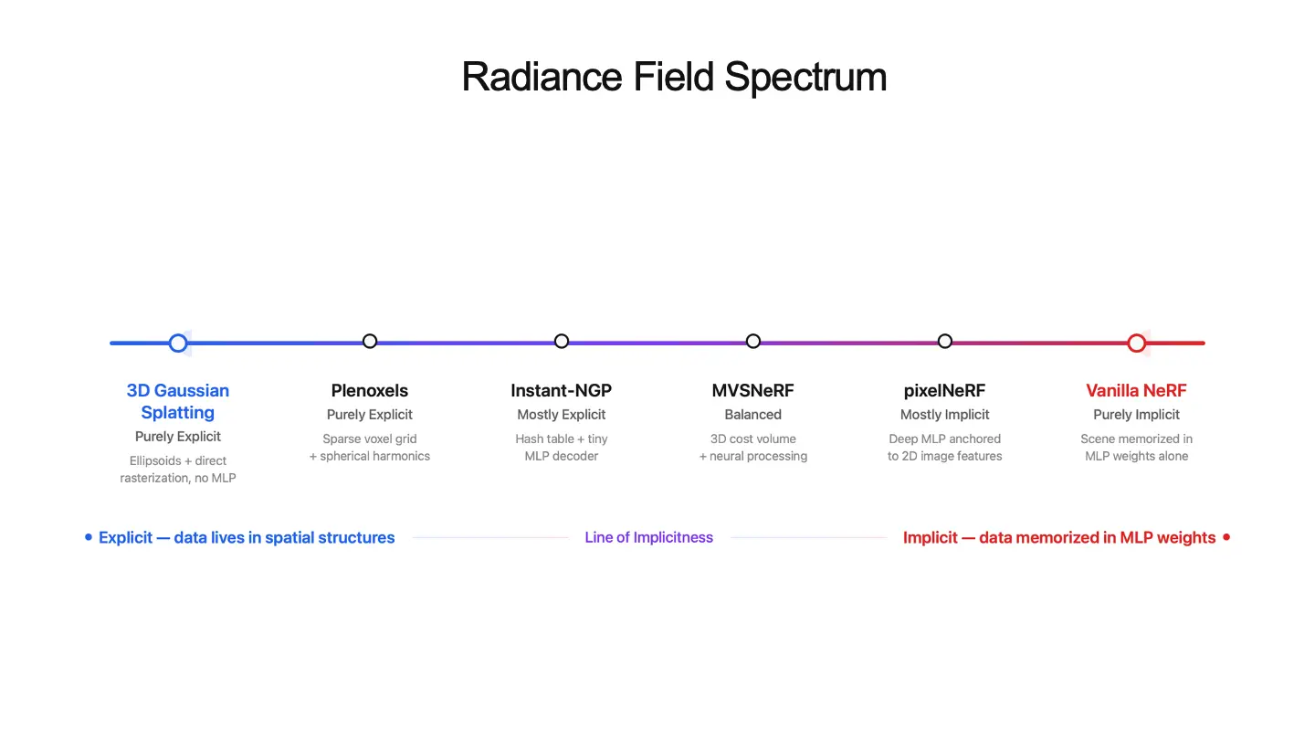
The Radiance Field Spectrum#

We can arrange these methods along a spectrum. The “Line of Implicitness” is defined by how the scene data is stored: Implicit methods store data in neural network weights (MLPs), while Explicit methods store data in spatial structures (grids, points, or Gaussians).

Here is how the methods highlighted in your article align from purely explicit to purely implicit:

Representation Type	Method	Key Mechanism	Why it fits there
Purely Explicit	3D Gaussian Splatting	3D Gaussians + Rasterization	No MLP involved. The “intelligence” is in the spatial primitives (ellipsoids) and their direct properties.
Purely Explicit	Plenoxels	Sparse Voxel Grid + Interpolation	Uses a grid and Spherical Harmonics. Explicitly skips neural networks to gain speed.
Hybrid (Mostly Explicit)	Instant-NGP	Hash Table + “Tiny” MLP	The bulk of the scene is in the Hash Table (explicit), but it still requires a very small MLP (implicit) to decode those features.
Hybrid (Balanced)	MVSNeRF	3D Cost Volume + 3D CNN/MLP	It builds an explicit 3D Cost Volume (from MVS) but uses implicit neural components to process and query that volume.
Hybrid (Mostly Implicit)	pixelNeRF	Image Features + Conditioned MLP	Relies on a deep MLP, but anchors it to explicit 2D image features (CNN maps) to allow for generalization.
Purely Implicit	Vanilla NeRF	Deep MLP (8+ layers)	The “Black Box.” No spatial data structure exists; the scene is entirely “memorized” within the weights of the MLP.

---

Summary of the Transition#

1. The Explicit End (3DGS / Plenoxels): You describe these as “physical 3D grids or clouds.” The computer simply “looks up” the color. This is why they achieve the real-time speeds you mentioned, as they avoid heavy math.
2. The Hybrid Middle (Instant-NGP / MVSNeRF): These methods represent the “Fast Adaptation” section of your note. They use data structures (Hash Tables or Cost Volumes) to do the heavy lifting, allowing the MLP to be “tiny” or just a “decoder.”
3. The Implicit End (Vanilla NeRF): As your note states, you can’t just “look up” a point here. You must feed coordinates into a “massive equation” (the MLP). This makes it highly data-efficient but computationally taxing, leading to the 122 million inferences per frame bottleneck you calculated.

This line effectively tracks the trade-off between Storage/Speed (Explicit) and Memory Efficiency/Continuity (Implicit).