A gentle introduction to Reinforcement Learning
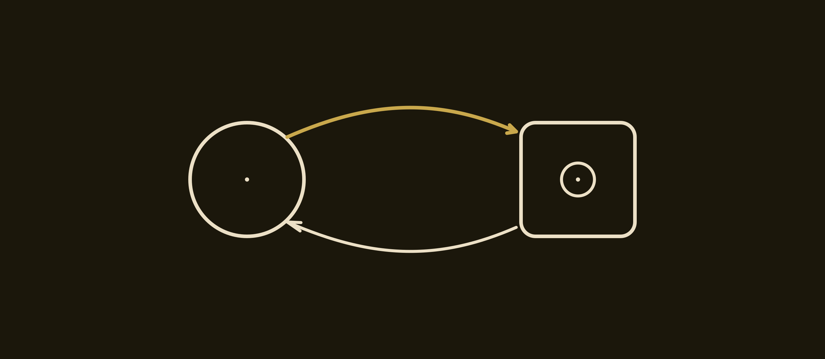
Reinforcement learning is trial-and-error learning: an agent takes actions in an environment to maximize cumulative reward. The math backbone is the Markov Decision Process and the Bellman equation, which expresses a state's value recursively through its successors. Value-based methods estimate how good states (or state-action pairs) are — planning with dynamic programming when the model is known, learning from experience with Monte Carlo and Temporal Difference updates when it isn't — and act greedily with respect to those estimates (SARSA on-policy, Q-learning off-policy). Policy-based methods skip values and optimize the policy directly via the policy gradient theorem (REINFORCE), taming its high variance with a baseline.
Introduction#
Supervised learning learns from labeled examples and unsupervised learning finds structure in data. Reinforcement learning (RL) learns from consequences: an agent explores an environment, receives numerical rewards for its actions, and gradually figures out which behavior maximizes long-term return. It is the framework behind game-playing agents, robotics controllers, and the RLHF step that aligns modern language models.
This post builds RL from the ground up. We start with the core vocabulary and the two big architectural choices (what to optimize, whether to model the environment), formalize the problem through Markov processes up to (PO)MDPs, and then walk the two solution families: value-based methods — from dynamic programming through Monte Carlo and TD to SARSA and Q-learning — and policy-based methods, ending with REINFORCE and variance reduction.
RL characterization#
Core vocabulary#
- State (S): A snapshot of the environment at a specific moment. It is the information the agent uses to make a decision (e.g., the current board position in a game of chess, or the sensor readings of a robot).
- Action (A): The set of all possible moves the agent can make in a given state.
- Reward (R): The numerical feedback the agent receives from the environment after taking an action. The agent’s ultimate goal is to maximize cumulative reward over time.
- Policy ($\pi$): The agent’s strategy or “rulebook.” It is a mapping from states to actions
- Value Function ($V$): A prediction of future reward. While the reward is immediate, the value function estimates the total amount of reward an agent can expect to accumulate over the long run, starting from a specific state.
- Model: The agent’s internal representation of the environment.
Categorization by optimization target#
When designing an RL agent, the first major architectural choice is deciding what exactly the agent is trying to optimize and learn. We can break this down into three main approaches:
Value-based learning#
In a value-based approach, the agent completely ignores learning a direct policy focusing its effort on learning the optimal Value Function.
Policy-based learning#
Policy-based methods take the exact opposite approach. Instead of calculating the value of states, they directly optimize the policy ($\pi$).
Actor-critic#
Actor-Critic methods combine the strengths of value-based and policy-based approaches.
- The Actor: This is the policy mechanism. It decides which action to take based on the current state.
- The Critic: This is the value function. It observes the action taken by the Actor and evaluates how good or bad it was, providing feedback to help the Actor improve.
Categorization by environment dynamics#
The second major way to classify RL algorithms is based on whether the agent tries to understand the “physics” or “rules” of its environment.
Model-free RL#
In Model-Free RL, the agent relies entirely on trial-and-error experience. It does not try to build an internal Model of how the environment works.
Model-based RL#
In Model-Based RL, the agent actively tries to learn a predictive Model of the environment.
Markov processes#
The current state is a sufficient statistics to characterize the future. The future is independent of the past given the present.
A Markov Process (or Markov Chain) is a tuple $
- $S$ is a finite set of states $s_1, s_2, s_3, ...$
- $P$ is a state transition matrix, s.t. $P_{ss'} = P(S_{t+1}=s'|S_t=s)$
Markov reward process#
A Markov Reward Process (MRP) is a Markov chain with reward values, tuple $
A Markov Reward Process is a tuple $S, P, R, \gamma$
- $S$ is a finite set of states $s_1, s_2, s_3, ...$
- $P$ is a state transition matrix, s.t. $P_{ss'}^a = P(S_{t+1} = s'|S_{t} = s)$
- $R$ is a reward function, s.t. $R_s= \mathbb{E}[R_{t+1}|S_{t}= s]$
- $\gamma$ is a discount factor, $\gamma \in [0,1]$
Global return#
The return $G_t$ is the total discounted reward from time-step $t$.
$$G_t=R_{t+1}+\gamma_1*R_{t+2}+\gamma_2*R_{t+3}+…=\sum_{k=0}^∞ γ^k R_{t+k+1}$$Value function#
The state-value function $\nu(s)$ of a Markov Reward Process is the expected return starting from state $s$
$$\nu(s)= \mathbb{E}[G_{t}|S_{t}= s]=\mathbb{E}[\sum_{k=0}^∞ γ^k R_{t+k+1}|S_t = s]$$Bellman equation#
From the previous state-value function we can isolate $R_{t+1}$, $R_{t+2}$
$$\mathbb{E}[R_{t+1} + \gamma(R_{t+2} + \sum_{k=2}^∞ γ^k R_{t+k+1}|S_t = s)]$$We can replace $G_{t+1}$
$$\mathbb{E}[R_{t+1} + \gamma \space G_{t+1}|S_t = s]$$We can replace $v(s_{t+1})$
$$v(s)=\mathbb{E}[R_{t+1} + \gamma \space v(s_{t+1})|S_t = s]$$And divide the equation value in expectation of instantaneous reward $\textcolor{#c9a84c}{R_s=\mathbb{E}[R_{t+1}|S_t = s]}$ and the expected state-value of being in any state reachable from $𝑠$, $\textcolor{#ece0c6}{\mathbb{E}[\gamma \space v(s_{t+1})|S_t = s]}$
$$v(s) = \textcolor{#c9a84c}{\mathbb{E}[R_{t+1}|S_t = s]} + \textcolor{#ece0c6}{\mathbb{E}[\gamma \space v(s_{t+1})|S_t = s]}$$Giving the Bellman Equation for MRPs
$$v(s) = R_s + \gamma \sum_{S'}P_{ss'}v(s')$$That in matrix form is:
$$v = R + \gamma \space P \space v= (I - \gamma \space P)^{-1} R \space v$$Solving the linear Bellman Equation in directly requires computational complexity of $O(n^3)$, infeasible for large MRPs
Markov Decision Process#
A Markov Decision Process (MDP) is a Markov reward process with actions/decisions, tuple $
- $S$ is a finite set of states $s_1, s_2, s_3, ...$
- $A$ is a finite set of actions $a_1, a_2, a_3, ...$
- $P$ is a state transition matrix, s.t. $P_{ss'}^a = P(S_{t+1} = s'|S_{t} = s, A_t = a)$
- $R$ is a reward function, s.t. $R_s^a= \mathbb{E}[R_{t+1}|S_{t}= s, At = a]$
- $\gamma$ is a discount factor, $\gamma \in [0,1]$
Given a policy for an action $a$ and a state $s$
$$\pi(a,s) = P(A_t = a|S_t = s)$$The state sequence is a Markov Process $
The state-value function, $v^{\pi(s)}$, represents the expected return (total accumulated discounted reward) starting from state s and following policy $\pi$.
$$v^{\pi(s)}(s) = \mathbb{E}[G_t|S_{t}= s]$$The Action-Value Function, also known as Q-function, $Q^{\pi}(s, a)$ represents the expected return starting from state s, taking action a, and then strictly following policy $\pi$ thereafter.
$$Q^{\pi}(s, a) = \mathbb{E}_{\pi} [G_t | S_t = s, A_t = a]$$Building on prior analysis, decomposing constituents leads to the Bellman Expectation Equation.
$$v^{\pi}(s) = \sum_{a \in \mathcal{A}} \pi(a|s) \left( \mathcal{R}_s^a + \gamma \sum_{s' \in \mathcal{S}} \mathcal{P}_{ss'}^a v^{\pi}(s') \right)$$That in matrix form is:
$$v = R^{\pi} + \gamma \space P^{\pi} v^{\pi} = I - \gamma \space P^{-1} R \space v^{\pi}$$In a MDP we can find so an optimal policy, a policy that yields the highest possible expected return (value) for every single state in the environment.
A policy $\pi$ is considered better than or equal to another policy $\pi'$ if its expected return is greater than or equal to that of $\pi'$ for all states.
$$\pi \geq \pi' \iff V^{\pi}(s) \geq V^{\pi'}(s) \quad \forall s \in \mathcal{S}$$In any finite MDP, there is always at least one policy that is better than or equal to all other policies. This is the optimal policy, denoted by $\pi_*$. There can be more than one optimal policy, but they all share the exact same state-value function and action-value function.
Because all optimal policies achieve the best possible returns, they share the optimal state-value function, denoted as $v_{\pi *}(s)$:
$$v_{\pi *}(s) = \max_{\pi} v_{*}(s) \quad \forall s \in \mathcal{S}$$They also share the optimal action-value function, denoted as $Q_{\pi*}(s,a)$:
$Q_{\pi*}(s, a) = \max_{\pi} Q_{*}(s, a) \quad \forall s \in \mathcal{S}, a \in \mathcal{A}$
Once you know the optimal action-value function $Q_{\pi*}(s)$, finding an optimal policy is straightforward. For any state s, the optimal policy strictly chooses the action a that maximizes the $Q_{*}$ value:
$$\pi^*(a|s) = \begin{cases} 1 & \text{if } a = \arg\max_{a \in \mathcal{A}} Q^*(s, a) \\ 0 & \text{otherwise} \end{cases}$$Partially Observable Markov Decision Process#
A Partially Observable Markov Decision Process (POMDP) is a generalization of an MDP where the agent cannot directly observe the underlying state, tuple $\langle S, A, P, R, \Omega, Z, \gamma \rangle$
- $S$ is a finite set of states $s_1, s_2, s_3, \dots$
- $A$ is a finite set of actions $a_1, a_2, a_3, \dots$
- $P$ is a state transition matrix, s.t. $P_{ss'}^a = P(S_{t+1} = s' | S_t = s, A_t = a)$
- $R$ is a reward function, s.t. $R_s^a = \mathbb{E}[R_{t+1} | S_t = s, A_t = a]$
- $\Omega$ is a finite set of observations $o_1, o_2, o_3, \dots$
- $Z$ is an observation function, s.t. $Z_{s'o}^a = P(O_{t+1} = o | S_{t+1} = s', A_t = a)$
- $\gamma$ is a discount factor, $\gamma \in [0, 1]$
- Markov is memorylessness: the present state is a sufficient statistic for the future, which is what makes the recursive Bellman formulation possible.
- MRP → MDP → POMDP is a ladder of realism: add actions to get decisions, hide the state behind observations to get partial observability.
- The Bellman equation splits value into immediate reward plus discounted future value — solve it exactly in $O(n^3)$ for small problems, approximate it everywhere else.
- Optimality is well-defined: every finite MDP has at least one optimal policy, and all optimal policies share the same $v_*$ and $Q_*$.
- Knowing $Q_*$ makes the policy trivial: act greedily, $\pi^*(s) = \arg\max_a Q^*(s, a)$ — the whole value-based enterprise is about estimating $Q$ well enough for this to work.
Value-based RL#
In Value-Based Reinforcement Learning, the agent’s primary goal is to estimate the optimal value function $V^*(s)$ or action-value function $Q^*(s, a)$. Instead of searching for a policy directly, the agent learns how “good” it is to be in a certain state or to take a specific action, and then derives a policy based on those estimates.
- Learned Value Function: The agent approximates the expected return (cumulative future reward) for states or state-action pairs. This is typically done by solving the Bellman optimality equations.
- Implicit Policy: The policy $\pi$ is not explicitly stored or parameterized. Instead, it is derived from the value function—for example, by acting greedily with respect to the learned Q-values: $\pi(s) = \arg\max_{a} Q(s, a)$.
- Optimization Goal: The objective is to minimize the Bellman error, ensuring the estimated values converge to the true expected returns.
Model-Based Value-Based RL#
In Model-Based Value-Based RL, the agent has access to a “model” of the environment—specifically the transition dynamics $P(s'|s, a)$ and the reward function $R(s, a)$. Instead of learning purely through trial and error (like model-free methods), the agent can “plan” by computing the optimal value function using its knowledge of how the world works.
- The Role of the Model: The model allows the agent to predict the outcome of actions without actually performing them.
- Planning via DP: Dynamic Programming (DP) is the primary framework for this planning. It uses the model to recursively solve the Bellman equations.
- Efficiency: Because the dynamics are known, the agent can compute the optimal policy offline before ever interacting with the environment.
Dynamic Programming#
Dynamic programming assumes full knowledge of the MDP. This makes it a Model-Based approach, where the agent uses its internal representation of the environment’s physics (transitions and rewards) to calculate the best possible actions.
Requirements for Dynamic Programming#
- Optimal substructure
- Overlapping subproblems
MDPs satisfy both properties.
Prediction Task#
In a task of prediction, the goal is to evaluate a given policy.
- Input: MDP $(S, A, P, R, \gamma)$ and policy $\pi$, or MRP $(S, P, R, \gamma)$.
- Output: Value function $v_\pi$.
Control Task#
In a task of control, the goal is to find the best possible behavior.
- Input: MDP $(S, A, P, R, \gamma)$.
- Output: Optimal value function $v^*$ and optimal policy $\pi^*$.
Policy Iteration#
Policy Iteration is a method to find the optimal policy $\pi^*$ by alternating between two distinct steps:
Step 1: Policy Evaluation: Given a policy $\pi$, calculate the value function $v_\pi$ for all states. This is done by solving the Bellman expectation equation, often iteratively: $v_{k+1}(s) = \sum_{a \in A} \pi(a|s) \sum_{s', r} p(s', r | s, a) [r + \gamma v_k(s')]$
Step 2: Policy Improvement: Update the policy to be greedy with respect to the current value function $v_\pi$. We create a new policy $\pi'$ that selects the action that maximizes the expected return: $\pi'(s) = \arg\max_{a} q_\pi(s, a) = \arg\max_{a} \sum_{s', r} p(s', r | s, a) [r + \gamma v_\pi(s')]$
Convergence: The process repeats ($\pi_0 \xrightarrow{E} v_{\pi_0} \xrightarrow{I} \pi_1 \xrightarrow{E} v_{\pi_1} \dots \xrightarrow{I} \pi^* \xrightarrow{E} v^*$). Since a finite MDP has a finite number of policies, this process is guaranteed to converge to the optimal policy and optimal value function in a finite number of steps.
Value Iteration#
Value iteration finds the optimal policy by iteratively updating the value function toward the optimal value function $v^*$, without waiting for the policy to fully converge at each step. It is based on the Bellman Optimality Equation.
The Algorithm: In each iteration, the value of a state is updated by taking the maximum expected return over all possible actions: $v_{k+1}(s) = \max_{a \in A} \sum_{s', r} p(s', r | s, a) [r + \gamma v_k(s')]$
Key Characteristics:
- No Explicit Policy: Unlike policy iteration, there is no explicit policy evaluation step. The “policy” is implicitly updated by taking the
maxover actions. - Convergence: The algorithm converges to $v^*$ as $k \to \infty$. In practice, it stops when the maximum change in the value function between iterations is less than a small threshold $\epsilon$.
- Efficiency: It is often faster than policy iteration because it doesn’t require multiple passes for policy evaluation in every loop.
- No Explicit Policy: Unlike policy iteration, there is no explicit policy evaluation step. The “policy” is implicitly updated by taking the
Final Policy Extraction: Once the optimal value function $v^*$ is found, the optimal policy $\pi^*$ is extracted by acting greedily: $\pi^*(s) = \arg\max_{a} \sum_{s', r} p(s', r | s, a) [r + \gamma v^*(s')]$
Model-Free Value-Based RL#
Unlike Dynamic Programming, Model-Free RL does not require knowledge of the environment’s internal dynamics (the transition probabilities $P$ and the reward function $R$). Instead, the agent learns the value function directly from experience by interacting with the environment.
- Learning from Samples: The agent explores the environment, collecting samples of $(s, a, r, s')$. It uses these samples to estimate the expected return.
- The Need for $Q(s, a)$: In model-based settings, we can use $V(s)$ to decide on an action because we know where each action leads. In model-free settings, we typically learn the Action-Value function $Q(s, a)$, which allows the agent to choose the best action without needing to know the transition dynamics.
While Dynamic Programming is about Planning (computing a solution for a known MDP), Model-Free RL is about Learning (estimating a solution for an unknown MDP through trial and error).
Model-Free Prediction#
Prediction is the process of calculating the value function for a fixed policy.
Monte Carlo Prediction#
Monte Carlo (MC) methods are the simplest way to estimate value functions by learning directly from episodes of experience.
Monte Carlo methods learn the value function by averaging the returns observed after visiting a state. It only requires samples (sequences of states, actions, and rewards).
Key Characteristics:
- Learning from complete episodes: MC methods only update the value function after a complete episode has terminated. It is not suitable for continuing tasks.
- No Bootstrapping: MC does not estimate values based on other value estimates (unlike TD learning or DP). It uses the actual realized return $G_t$.
- High Variance, Zero Bias: Because $G_t$ depends on many random actions and transitions throughout an episode, the variance is high. However, the estimate is unbiased.
The Algorithm: MC uses the simplest possible idea, value = mean return across episodes:
$$V(s) \approx \frac{1}{N(s)} \sum_{i=1}^{N(s)} G_{i,t}$$Or, expressed as the expected return:
$$V(s) = \mathbb{E}_\pi [G_t \mid S_t = s]$$Where:
- $V(s)$ is the estimated value of state $s$.
- $G_{i,t}$ is the return following the $t$-th step in the $i$-th episode.
- $N(s)$ is the total number of times state $s$ has been visited.
To estimate $v_\pi(s)$, the agent:
- Follows policy $\pi$ to generate an episode: $S_0, A_0, R_1, S_1, A_1, R_2, \dots, S_T$.
- Calculates the return $G_t = \sum_{k=0}^{T-t-1} \gamma^k R_{t+k+1}$.
- Updates the average for state $S_t$: $$V(S_t) \leftarrow V(S_t) + \alpha (G_t - V(S_t))$$ where $\alpha$ is a constant step-size (learning rate).
First-Visit vs. Every-Visit MC#
- First-Visit MC: Only the first time a state $s$ is visited in an episode is used to update $V(s)$.
- Every-Visit MC: Every time a state $s$ is visited in an episode, the return following that visit is used to update $V(s)$.
Temporal Difference (TD) Learning#
Temporal Difference (TD) learning is a combination of Monte Carlo (MC) ideas and Dynamic Programming (DP) ideas. Like MC, TD can learn directly from raw experience without a model of the environment’s dynamics. Like DP, TD updates estimates based in part on other learned estimates, without waiting for a final outcome (a process called bootstrapping).
TD learning updates the value function after every single step ($S_t, A_t, R_{t+1}, S_{t+1}$), rather than waiting until the end of an episode.
The simplest form of TD learning, known as TD(0), updates the state-value $V(S_t)$ toward a TD Target:
$$V(S_t) \leftarrow V(S_t) + \alpha [ \underbrace{R_{t+1} + \gamma V(S_{t+1})}_{\text{TD Target}} - V(S_t) ]$$Where:
- TD Target: $R_{t+1} + \gamma V(S_{t+1})$ is the estimate of the return.
- TD Error ($\delta_t$): The difference between the estimated return and the current value: $$\delta_t = R_{t+1} + \gamma V(S_{t+1}) - V(S_t)$$
Key Characteristics:
- Bootstrapping: TD updates its estimate $V(S_t)$ based on another estimate $V(S_{t+1})$.
- Online Learning: TD can learn from incomplete sequences and is suitable for continuous tasks that never end.
- Low Variance, Some Bias: Because it depends on only one random step ($R_{t+1}, S_{t+1}$) rather than a whole sequence, it has lower variance than MC. However, it is biased toward the initial (possibly wrong) value estimates.
Comparison: MC vs. TD#
| Feature | Monte Carlo (MC) | Temporal Difference (TD) |
|---|---|---|
| Update Timing | End of episode | Every step |
| Requirement | Complete episodes | Can learn from incomplete episodes |
| Bias/Variance | Zero Bias / High Variance | Some Bias / Low Variance |
| Equation | $V(S_t) \leftarrow V(S_t) + \alpha (G_t - V(S_t))$ | $V(S_t) \leftarrow V(S_t) + \alpha (R_{t+1} + \gamma V(S_{t+1}) - V(S_t))$ |
| Efficiency | Slower to converge | Usually faster to converge |
| Markov Properties | not exploited | exploited |
Model-Free Control#
Control is the process of finding the optimal policy that maximizes the total reward.
On-Policy#
In on-policy control, the agent learns about the policy it is currently following. A fundamental shift in model-free control is the move from state-value functions to action-value functions.
Why use $Q(s, a)$ instead of $V(s)$?
- Greedy policy improvement over $V(s)$ requires a model of the MDP. To choose the best action, the agent needs to know the transition probabilities and reward function: $$\pi'(s) = \arg \max_{a \in \mathcal{A}} \left( \mathcal{R}_s^a + \gamma \sum_{s' \in \mathcal{S}} \mathcal{P}_{ss'}^a V(s') \right)$$
- Greedy policy improvement over $Q(s, a)$ is model-free. The agent can choose the best action simply by looking at the learned values, without needing to know the environment’s “physics”: $$\pi'(s) = \arg \max_{a \in \mathcal{A}} Q(s, a)$$
Monte Carlo Control#
To find the optimal policy without a model, we must estimate Action-Values $Q(s, a)$ instead of State-Values $V(s)$. If we only have $V(s)$, we would need the transition dynamics $P(s'|s, a)$ to choose the best action.
- Policy Evaluation: Estimate $Q \approx q_\pi$ using Monte Carlo.
- Policy Improvement: Improve the policy by acting greedily with respect to the current Q-table: $$\pi(s) = \arg\max_{a} Q(s, a)$$
Since MC relies on experience, it might never “see” the best actions if the policy becomes deterministic too quickly. To solve this, we use $\epsilon$-greedy exploration:
- With probability $1 - \epsilon$, choose the best action (greedy).
- With probability $\epsilon$, choose a random action.
SARSA: State-Action-Reward-State-Action#
SARSA is an on-policy TD control algorithm. Its name represents the quintuple of events $(S_t, A_t, R_{t+1}, S_{t+1}, A_{t+1})$ that occur in a single update cycle.
- The Concept: The agent starts in state $S$, takes action $A$, receives reward $R$, and lands in state $S'$. Then, it chooses the next action $A'$ according to its current policy (e.g., $\epsilon$-greedy). It uses the value of that next state-action pair $Q(S', A')$ to update the current one.
- Update Rule: $$Q(S, A) \leftarrow Q(S, A) + \alpha [R + \gamma Q(S', A') - Q(S, A)]$$
- Key Characteristic: Because $A'$ is chosen using the same policy $\pi$ that generated $A$, SARSA is on-policy. It accounts for the exploration (the “mistakes”) the agent might make while following an $\epsilon$-greedy policy.
SARSA Algorithm Loop:
- Initialize $Q(s, a)$ arbitrarily.
- For each episode:
- Initialize $S$.
- Choose $A$ from $S$ using policy derived from $Q$ (e.g., $\epsilon$-greedy).
- For each step of episode:
- Take action $A$, observe $R, S'$.
- Choose $A'$ from $S'$ using policy derived from $Q$.
- $Q(S, A) \leftarrow Q(S, A) + \alpha [R + \gamma Q(S', A') - Q(S, A)]$
- $S \leftarrow S'; A \leftarrow A';$
- Until $S$ is terminal.
Off-Policy Control#
In off-policy learning, we evaluate or improve a target policy $\pi(a|s)$ while following a different behavior policy $\mu(a|s)$.
- Target Policy ($\pi$): The policy the agent is trying to learn (usually the optimal greedy policy).
- Behavior Policy ($\mu$): The policy used to generate the agent’s experience (usually an exploratory policy like $\epsilon$-greedy).
Why use Off-Policy?
- Learn from observing humans or other agents.
- Re-use experience generated from old policies (Experience Replay).
- Learn about the optimal policy while still exploring the environment.
Q-Learning#
Q-Learning is the most famous off-policy TD control algorithm. Unlike SARSA, which uses the action $A'$ actually chosen by the behavior policy, Q-Learning assumes the agent will follow the best possible action in the next state.
- The Concept: The agent is in state $S$, takes action $A$, receives reward $R$, and moves to $S'$. To update $Q(S, A)$, it looks at $S'$ and picks the action that has the maximum $Q$-value, regardless of what action the behavior policy actually chooses next.
- Update Rule: $$Q(S, A) \leftarrow Q(S, A) + \alpha [R + \gamma \max_{a'} Q(S', a') - Q(S, A)]$$
- Key Characteristic: It is off-policy because the update uses the maximum value over all possible actions ($\max_{a'} Q(S', a')$), which represents the greedy target policy, even if the agent actually takes an exploratory (non-greedy) action next.
Q-Learning Algorithm Loop:
- Initialize $Q(s, a)$ arbitrarily.
- For each episode:
- Initialize $S$.
- For each step of episode:
- Choose $A$ from $S$ using policy derived from $Q$ (e.g., $\epsilon$-greedy).
- Take action $A$, observe $R, S'$.
- $Q(S, A) \leftarrow Q(S, A) + \alpha [R + \gamma \max_{a'} Q(S', a') - Q(S, A)]$
- $S \leftarrow S'$
- Until $S$ is terminal.
- Planning ≠ learning: dynamic programming computes a solution for a known MDP, while model-free methods estimate one for an unknown MDP through trial and error.
- MC vs. TD is bias vs. variance: Monte Carlo waits for full episodes (unbiased, high variance), TD bootstraps every step (biased, low variance, works for continuing tasks).
- Model-free control needs $Q$, not $V$: greedy improvement over $V(s)$ requires transition dynamics, while $\arg\max_a Q(s, a)$ needs none.
- SARSA vs. Q-learning is honesty vs. optimism: SARSA evaluates the exploratory policy it follows (on-policy), Q-learning targets the greedy policy while exploring (off-policy).
- $\epsilon$-greedy is the price of learning: without exploration, Monte Carlo control would never discover the actions its greedy policy never tries.
Policy-based RL#
Policy Objective Functions#
To optimize the policy $\pi_\theta$, we need a scalar measure to evaluate its quality $J(\theta)$. Depending on the type of environment, we define $J(\theta)$ differently:
Episodic Environments: Start Value#
In environments that have a defined start state $s_1$ and end in a terminal state, we aim to maximize the expected return from the beginning.
$$J_1(\theta) = V^{\pi_\theta}(s_1) = \mathbb{E}_{\pi_\theta}[G_1]$$- This represents the expected cumulative reward when starting the episode at $s_1$.
Continuing Environments: Average Value or Reward#
In environments that run indefinitely, we look at the long-term performance.
- Average Value: The mean value of states, weighted by how often we visit them. $$\bar{J}_V(\theta) = \sum_s d^{\pi_\theta}(s) V^{\pi_\theta}(s)$$
- Average Reward (per time-step): The expected immediate reward we receive at any given step. $$\bar{J}_R(\theta) = \sum_s d^{\pi_\theta}(s) \sum_a \pi_\theta(a|s) \mathcal{R}_s^a$$ This measures how much immediate reward the agent can “harvest” on average.
The Stationary Distribution $d^{\pi_\theta}(s)$#
In the equations above, $d^{\pi_\theta}(s)$ is the stationary distribution of the Markov chain under policy $\pi_\theta$.
- It represents the probability of being in state $s$ in the long run (as $t \to \infty$), regardless of the starting state.
- It satisfies the condition: $d^{\pi_\theta}(s) = \sum_{s'} d^{\pi_\theta}(s') \mathcal{P}_{s's}^a$.
Finite Difference Policy Gradient#
Before looking at analytical gradients, the simplest way to estimate the gradient of the objective function $J(\theta)$ is through numerical differentiation. This is a “black-box” approach because it doesn’t require the policy to be differentiable or even know how the environment works.
The Concept#
We perturb each parameter $\theta_k$ by a small amount $\epsilon$ and observe how the objective function $J(\theta)$ changes. This allows us to estimate the partial derivative for each dimension of the parameter vector.
The Formula#
For each dimension $k \in [1, n]$ of the parameters $\theta$:
$$\frac{\partial J(\theta)}{\partial \theta_k} \approx \frac{J(\theta + \epsilon u_k) - J(\theta)}{\epsilon}$$Where $u_k$ is a unit vector with 1 in the $k$-th component and 0 elsewhere.
A more accurate (but twice as expensive) estimate is the symmetric difference:
$$\frac{\partial J(\theta)}{\partial \theta_k} \approx \frac{J(\theta + \epsilon u_k) - J(\theta - \epsilon u_k)}{2\epsilon}$$Policy Gradient Theorem#
To maximize $J(\theta)$, we use Gradient Ascent:
$$\theta_{t+1} = \theta_t + \alpha \nabla_\theta J(\theta_t)$$The Policy Gradient Theorem provides an analytical expression for the gradient without requiring the derivative of the state distribution:
$$\nabla_\theta J(\theta) = \mathbb{E}_{\pi_\theta} [\nabla_\theta \log \pi_\theta(a|s) Q^{\pi_\theta}(s, a)]$$- Score Function: $\nabla_\theta \log \pi_\theta(a|s)$ tells us how to adjust $\theta$ to increase the probability of action $a$.
- Weight: $Q^{\pi_\theta}(s, a)$ tells us how “good” that action was.
REINFORCE (Monte Carlo Policy Gradient)#
REINFORCE is the simplest policy gradient algorithm. It uses the actual return $G_t$ from an episode as an unbiased estimate of $Q^{\pi_\theta}(s, a)$.
The Update Rule:
$$\theta \leftarrow \theta + \alpha \nabla_\theta \log \pi_\theta(S_t, A_t) G_t$$Algorithm Loop:
- Initialize policy parameter $\theta$ arbitrarily.
- For each episode $\{S_1, A_1, R_2, \dots, S_T\}$ generated by $\pi_\theta$:
- For each step $t = 1, \dots, T-1$:
- $G \leftarrow$ return from step $t$.
- $\theta \leftarrow \theta + \alpha \gamma^t G \nabla_\theta \log \pi_\theta(A_t|S_t)$
- For each step $t = 1, \dots, T-1$:
Reducing Variance with a Baseline#
The main drawback of REINFORCE is high variance. We can reduce this by subtracting a baseline $B(s)$ (usually the state-value function $V(s)$) from the return:
$$\nabla_\theta J(\theta) = \mathbb{E}_{\pi_\theta} [\nabla_\theta \log \pi_\theta(a|s) (G_t - B(s))]$$- Pick the objective that matches the task: start-state value for episodic environments, average value or average reward for continuing ones.
- Finite differences are a black-box fallback: no differentiability needed, but one noisy evaluation per parameter makes them expensive.
- The policy gradient theorem removes the hard part: the gradient needs no derivative of the stationary state distribution, just $\nabla_\theta \log \pi_\theta(a|s)$ weighted by $Q(s, a)$.
- REINFORCE is unbiased but shaky: using the raw return $G_t$ as the weight gives high variance, which is why a baseline $B(s)$ — typically $V(s)$ — is subtracted without introducing bias.
References#
- Sutton & Barto — Reinforcement Learning: An Introduction (2nd ed.): The canonical textbook; chapters on MDPs, dynamic programming, Monte Carlo, TD, and policy gradients mirror this post’s arc.
- David Silver — UCL Course on Reinforcement Learning: Lecture videos covering the same progression from Markov processes to value-based and policy-based control.
- OpenAI Spinning Up in Deep RL: A practical companion for taking these tabular ideas into deep function approximation.