Tokenizers are easy!

Your LLM has never read a single word. It reads tokens — and the way text gets chopped up matters more than you'd think. Splitting on spaces explodes the vocabulary and chokes on anything outside English. The fix? Byte-Pair Encoding: start from raw bytes, greedily merge the most frequent pairs, repeat. Simple idea, nasty bottleneck — the naive version scans every word on every merge, costing O(V × M). An inverted index cuts that to only the words that matter (~17× faster). Pair it with a max-heap and the speedup compounds to 85× at full vocabulary. All implementations are open-source.
Introduction#
If you’re into Artificial Intelligence recently, you’ve surely heard that prior to adding positional embedding, computing attention, and so on, transformers convert words into embeddings. You’ve also likely heard that this is a simplification because, more precisely, sentences are first converted into tokens.
Tokenization basics#
We can consider tokens as the smallest units of the input provided to the architecture, and the specific tokens generated for a given sentence will vary depending on the tokenizer used. Let’s look an example using OpenAI Tokenizer, the trivial sentence I will try to tokenize is: “Hi! I’m Giacomo and i’m trying to understand what tokenizers are.” 13 words. The output for latest OpenAI models is:
Word-Level tokenization hurdles#
So why don’t tokenizers just split sentences into words? It seems like the best choice for all. Well, it’s not a free lunch. Most importantly, the model’s vocabulary is constrained by the embedding matrix, which could “explode” if there are too many words. In English there are hundreds of thousands of words and maybe this amount could also be managed but if you’re doing a multi-language model you’re hopeless. Furthermore, using a vocabulary intrinsically “fixed” without subwords led to a lack of representation when there are out-of-vocabulary (OOV) words. If the model doesn’t have “bio-luminescence” in its dictionary, it marks it as [UNK] (Unknown) and so that word becomes a blank space while with subwords it could be easily represented as bio + luminescence.
Subwords for the win#
Languages are also intrinsically modular: Consider the word “unhappily”. With a single token the model sees one unique string, while with subwords the model sees un (negation) + happy(emotion) + ly (adverb). By breaking words down, the model learns that the prefix un- usually means “not,” regardless of which word it’s attached to. This makes the AI much better at understanding grammar and relationships between words. A token can serve multiple purposes, and building upon a common prefix can enhance the model’s capacity to understand the semantic field of that word. Using same prefix for more words makes feasible the computation and keep the embedding matrix contained.
Vocabulary grows with the internet#
Taking a look at the second split, GPT-3 considered the word “tokenizers” as two tokens: " token" and “izers”. Thus, the concept of “token”, encoded as 11241, can be used on its own but also contributes to the concept of “tokenizers” when followed by “izers”. This is a purely statistical trade-off: if a word appears frequently, it may make sense to assign it a dedicated token; otherwise, the word may be split into smaller tokens to represent the whole concept.
Indeed, if we examine the first tokenization of the sentence, we see that “tokenizers” is treated as a single token. This could be due to various reasons. One plausible hypothesis is that the source on which the latest tokenizer was trained likely had more examples of “tokenizers”, as the word became more prevalent between the training of GPT-3 and GPT-5, driven by the rise of AI.
This reasoning applies to tokenizer models based on word occurrences in real-world data, which are commonly referred to as Byte-Pair Encoding (BPE) tokenizers due to the algorithm used to train them. Before introducing BPE, it is helpful to cover some basics that stem from common techniques used in classic NLP tasks.
Character-Level Encoding#
First idea that can come out is to encode each character as an index in our vocabulary of fixed size. Unicode performs this encoding by mapping every distinct character across 168 different scripts to a unique integer code point. For example, the Latin character “s” is assigned the index 115 (U+0073), while the Chinese character “牛” is assigned 29275.
However, using raw Unicode code points as our model’s token vocabulary presents massive computational hurdles. We cannot simply encode each character as a single token due to a prohibitively large vocabulary, indeed with nearly 155,000 characters defined in the standard, the embedding matrix required for the model’s input and output layers would be enormous bloating the model’s memory footprint and slowing down training. Another problem is data sparsity: A 150K+ vocabulary would be less functional in practice. How many times will an user use a specific emoji? Not enough to allocate a token. While a token for the letter “e” might appear billions of times in an English training corpus, thousands of obscure symbols, historical scripts or rare emojis might only appear a handful of times. The model would struggle to learn meaningful mathematical representations for these rare characters due to a lack of context and training examples.
Byte-Level Encoding#
To achieve necessary computational improvements, modern language models abandon this 1-to-1 character mapping dropping down to a much smaller, denser foundational layer using byte-level encodings like UTF-8. The key idea here is that by converting text into UTF-8, we restrict the base vocabulary to just 256 distinct byte values (integers from 0 to 255). As we already mentioned above, any Unicode character can be translated into a sequence of these bytes, out-of-vocabulary issues are entirely eliminated. From this highly manageable 256-item vocabulary, algorithms like Byte-Pair Encoding (BPE) systematically merge the most frequent byte sequences into larger “subword” tokens.
Now that we have the basics covered, we can look at how BPE builds on top of byte-level encoding to produce a practical, efficient vocabulary.
- Fewer tokens = less compute: each token maps to a fixed-size embedding regardless of its length, so a compact tokenization directly reduces model cost.
- Word-level vocabularies don't scale: hundreds of thousands of words per language would explode the embedding matrix, and any unseen word collapses to [UNK].
- Subwords capture morphology: splitting "unhappily" into un + happy + ly lets the model generalise prefixes and suffixes across words it has never seen whole.
- Token boundaries are statistical, not linguistic: a word gets its own token only when it appears frequently enough in the training corpus — "tokenizers" earned a single token between GPT-3 and GPT-5 simply because the internet started using it more.
- Character-level Unicode is impractical: ~155 000 code points create a sparse, memory-heavy vocabulary where rare symbols never accumulate enough examples to learn from.
- UTF-8 bytes are the right base layer: any text maps losslessly onto 256 byte values, eliminating out-of-vocabulary issues while keeping the seed vocabulary tiny enough for BPE to build on top of.
Byte Pair Encoding#
The byte pair encoding algorithm isn’t a novelty in computer science, it’s been described by Philippe Gage in 1994 as a new algorithm for data compression. Then in 2016, Sennrich et Al. proposed to introduce this tokenization into NLP, in order to address problems described above. BPE starts with a vocabulary of individual bytes, then repeatedly finds the most frequent adjacent pair of tokens across the corpus, merges them into a single new token, and adds that token to the vocabulary. This process continues until the vocabulary reaches the desired size.

Nowadays, code is more of a commodity than ever before, but I still feel that spending time on algorithms and implementation details makes sense. The devil is in the details, especially with AI-generated code, so I will provide in this section an overview of hand-written BPE algorithms in an incremental fashion, from naive to most optimized.
Pre-Tokenization#
Pretokenization is a coarse-grained tokenization step that runs before training begins. Rather than operating directly on the raw byte stream of the corpus, we first split the text into surface words and count how often each unique word appears.
This frequency table is the only thing BPE ever sees avoiding to touch the original corpus again.
Pretokenization solves two problems at once. First, it avoids scanning the entire corpus on every merge step: instead of walking through raw text repeatedly, we count word frequencies once up front and represent each unique word as a sequence of bytes with an associated count.
So basically if we would know how often two bytes appear adjacent, we simply multiply by the word’s frequency, e.g. if "text" appears 10,000 times, we credit the t/e pair 10,000 at once. Second, it prevents merges from crossing word boundaries, which would produce tokens like dog! and dog. that are semantically identical but would receive completely different IDs. By treating each surface word as an isolated unit, BPE merges only happen within words, keeping the resulting vocabulary linguistically coherent.
To split text into surface words, I relied on the GPT-2 pretokenization regex:
PAT = '(?:[sdmt]|ll|ve|re)| ?\p{L}+| ?\p{N}+| ?[^\s\p{L}\p{N}]+|\s+(?!\S)|\s+
This regex expression is based on the English language and makes it highly useful for our future training on the TinyStories dataset.
| Pattern | Description | Examples |
|---|---|---|
(?:[sdmt]|ll|ve|re) | Matches common English language endings | 's, 't, 'll, 've |
?\p{L}+ | Matches a run of Unicode letters, optionally preceded by a single space. | apple, café, π |
?\p{N}+ | Matches a run of Unicode numbers/digits, optionally preceded by a single space. | 123, 45 |
[^\s\p{L}\p{N}]+ | Matches a run of characters that are not whitespace, letters, or numbers. | !!!, :), @#$ |
\s+(?!\S) | Matches whitespace characters that are not followed by any non-space character. | |
\s+ | Matches any other leftover whitespace sequences. | \t, \n, |
We are ready to dive into algorithms now.
Naive#
A first naive idea is to scan the entire corpus, merge the most frequent adjacent pair and recount the occurrences with the pair encoded as a single token on every step until we reach the desired vocabulary size. A first optimization can be to maintain a running frequency table of all adjacent token pairs, pick the most frequent one, merge it into a single new token, and update the frequency table by scanning every word in the corpus and then repeating until the desired vocabulary size is reached. The algorithm is conceptually simple:
- Scan
pair_counts, a flat dict mapping every adjacent token pair(a, b)to its aggregate frequency across all words and pick the maximum with. This isO(P)where P is the number of distinct pairs. - Assign the next available ID
iand recordtokens[i] = tokens[a] + tokens[b]. - Iterate over all words in the corpus. For each word, do a linear scan of its current token sequence and replace every occurrence of
(a, b)withi. While doing so, surgically updatepair_countsin-place: the three affected pairs —(prev, a),(a, b), and(b, next)— are decremented, and their replacements(prev, i)and(i, next)are incremented. This avoids a full recount from scratch. - Repeat for
num_mergessteps, or until no pair has positive frequency.
The cost is O(V × M): V words scanned per merge, M merges total. Later we will discover that Step 3 is the bottleneck, indeed, even if only a handful of words actually contain the pair (a, b), you visit every word anyway.
Wall time#
| Merges | Naive |
|---|---|
| 500 | 17.97 s |
| 1 000 | 34.59 s |
| 2 000 | 66.64 s |
| 5 000 | 156.40 s |
| 9 743 | 300.80 s |
Throughput (merges / second)#
| Merges | Naive |
|---|---|
| 500 | 28 |
| 1 000 | 29 |
| 2 000 | 30 |
| 5 000 | 32 |
| 9 743 | 32 |
Maybe a Max-Heap?#
That scan for max within the pairs dict in O(P) sounds suspicious, can’t we arrange a data structure where we can extract the max in O(1)?
Well, almost. For a general priority queue, an O(log P) extraction is the practical standard;
no common structure supports O(1) worst-case extraction.
We could achieve O(1) amortized extraction with a bucket queue, an array indexed by frequency, but this requires knowing (or capping) the maximum possible frequency upfront to size the buckets. Memory usage scales with that maximum frequency, not with the number of distinct pairs.
For a tokenizer trained on a large corpus, a single pair’s frequency can reach into the millions, making a naive bucket queue highly memory-intensive in practice. Instead, here we can use a max-heap, that is simpler and scales better in practice. Main properties for this use case:
- Extract the best pair in O(log P)
- Memory proportional to the number of distinct pairs
- Handles arbitrarily large counts without preallocation


The complication is keeping the heap consistent. When a merge updates pair_counts, you can’t efficiently remove or modify existing heap entries.
The solution is lazy deletion: rather than fixing stale entries, you just push the new count onto the heap and skip any popped entry whose stored frequency doesn’t match the current pair_counts value.
The heap may accumulate stale entries, but they get filtered out naturally on pop.
Wall time#
| Merges | Naive | Heap |
|---|---|---|
| 500 | 17.97 s | 20.20 s |
| 1 000 | 34.59 s | 38.01 s |
| 2 000 | 66.64 s | 68.87 s |
| 5 000 | 156.40 s | 151.46 s |
| 9 743 | 300.80 s | 267.48 s |
Speedup vs. Naive#
| Merges | Naive | Heap |
|---|---|---|
| 500 | 1.0× | 0.9× |
| 1 000 | 1.0× | 0.9× |
| 2 000 | 1.0× | 1.0× |
| 5 000 | 1.0× | 1.0× |
| 9 743 | 1.0× | 1.1× |
Throughput (merges / second)#
| Merges | Naive | Heap |
|---|---|---|
| 500 | 28 | 25 |
| 1 000 | 29 | 26 |
| 2 000 | 30 | 29 |
| 5 000 | 32 | 33 |
| 9 743 | 32 | 36 |
As I mentioned before, Heap doesn’t give so much gains alone, it shines a bit only on big numbers. Let’s try to address the true bottleneck.
Inverted Index#
The inverted index version attacks the other bottleneck: which words get scanned.
The key addition is pair_to_words: an inverted index mapping each pair (a, b) to the set of words that currently contain it.
When merging (a, b), instead of iterating over all words in the corpus, you only visit pair_to_words[(a, b)].
If a pair appears in 50 out of 100,000 words, you touch 50 words instead of 100,000.
The tradeoff is that pair_to_words must be kept in sync after each merge. After rewriting a word’s sequence, all its old pairs are removed from the index and all new pairs are added.
This is an O(L) operation per affected word (L being the sequence length), which is cheap compared to the scanning it avoids.
Best-pair selection is still max() over pair_counts, an O(P).
So the indexed version trades the word scan cost for an index maintenance cost, while leaving the other bottleneck untouched.
Wall time#
| Merges | Naive | Heap | Inverted Index |
|---|---|---|---|
| 500 | 17.97 s | 20.20 s | 1.04 s |
| 1 000 | 34.59 s | 38.01 s | 2.14 s |
| 2 000 | 66.64 s | 68.87 s | 5.13 s |
| 5 000 | 156.40 s | 151.46 s | 17.88 s |
| 9 743 | 300.80 s | 267.48 s | 45.64 s |
Speedup vs. Naive#
| Merges | Naive | Heap | Inverted Index |
|---|---|---|---|
| 500 | 1.0× | 0.9× | 17.2× |
| 1 000 | 1.0× | 0.9× | 16.1× |
| 2 000 | 1.0× | 1.0× | 13.0× |
| 5 000 | 1.0× | 1.0× | 8.7× |
| 9 743 | 1.0× | 1.1× | 6.6× |
Throughput (merges / second)#
| Merges | Naive | Heap | Inverted Index |
|---|---|---|---|
| 500 | 28 | 25 | 480 |
| 1 000 | 29 | 26 | 467 |
| 2 000 | 30 | 29 | 390 |
| 5 000 | 32 | 33 | 280 |
| 9 743 | 32 | 36 | 213 |
The natural next step is to combine both optimizations: use the inverted index to limit the word scan and the heap to speed up best-pair selection, which is exactly what our last optimization does.
Inverted Index + Heap#
The inverted heap version simply combines both optimizations.
Recall the two bottlenecks in the naive algorithm:
- Finding the best pair — O(P) linear scan over
pair_counts - Rewriting words — O(V) scan over all words, even those that don’t contain the pair
The heap fixes (1). The inverted index fixes (2). Together they give you O(log P) best-pair selection and O(W) word rewriting per merge, where W is the number of words actually containing the pair.
The only added complexity over using either optimization alone is that both data structures must be kept in sync during the merge step: pair_to_words is updated after each word rewrite (old pairs discarded, new pairs added), and the heap receives a new push for every pair_counts entry that changes. Both are O(L) per affected word, where L is the token sequence length.
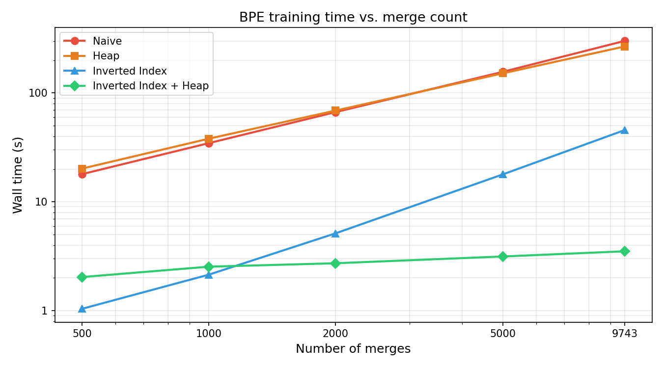
Wall time#
| Merges | Naive | Heap | Inverted Index | Inv. Index + Heap |
|---|---|---|---|---|
| 500 | 17.97 s | 20.20 s | 1.04 s | 2.04 s |
| 1 000 | 34.59 s | 38.01 s | 2.14 s | 2.54 s |
| 2 000 | 66.64 s | 68.87 s | 5.13 s | 2.73 s |
| 5 000 | 156.40 s | 151.46 s | 17.88 s | 3.15 s |
| 9 743 | 300.80 s | 267.48 s | 45.64 s | 3.51 s |
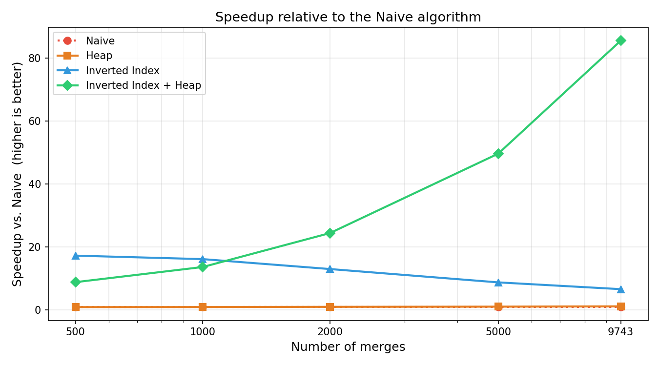
Speedup vs. Naive#
| Merges | Naive | Heap | Inverted Index | Inv. Index + Heap |
|---|---|---|---|---|
| 500 | 1.0× | 0.9× | 17.2× | 8.8× |
| 1 000 | 1.0× | 0.9× | 16.1× | 13.6× |
| 2 000 | 1.0× | 1.0× | 13.0× | 24.4× |
| 5 000 | 1.0× | 1.0× | 8.7× | 49.7× |
| 9 743 | 1.0× | 1.1× | 6.6× | 85.6× |
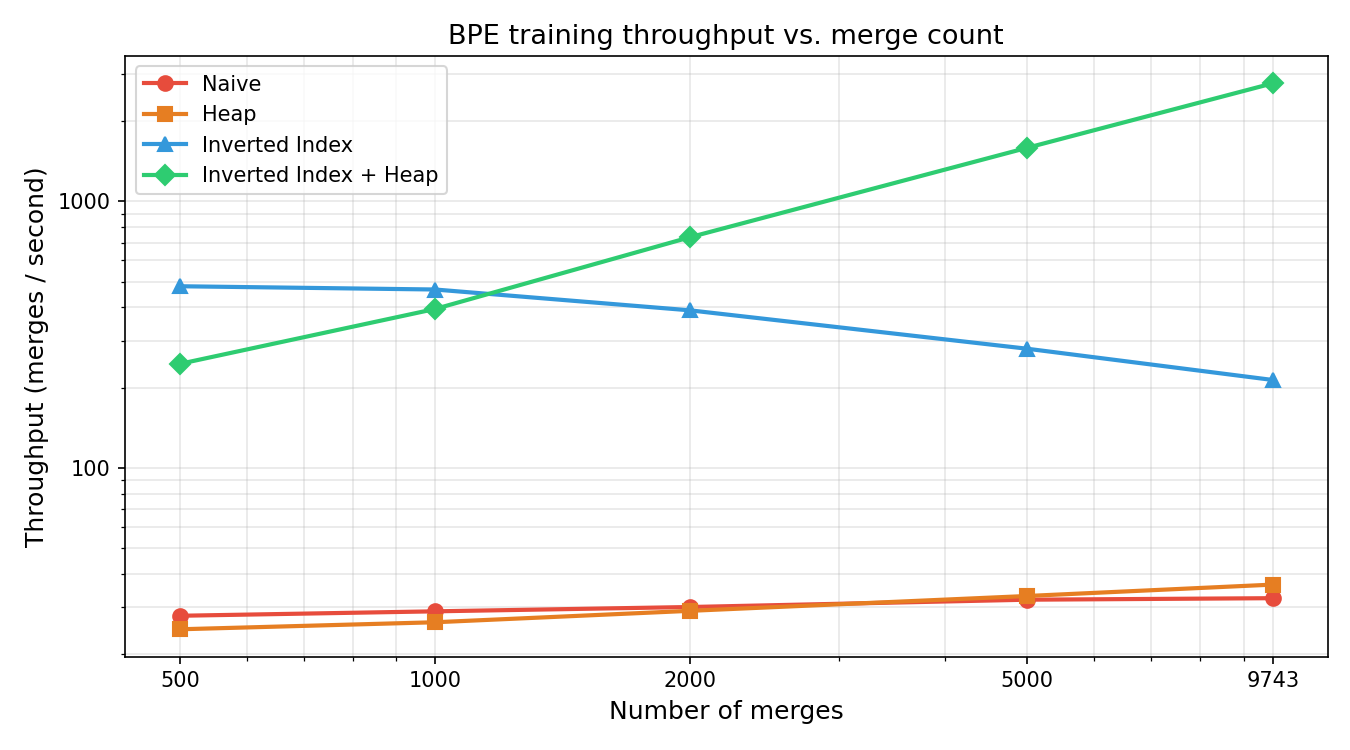
Throughput (merges / second)#
| Merges | Naive | Heap | Inverted Index | Inv. Index + Heap |
|---|---|---|---|---|
| 500 | 28 | 25 | 480 | 245 |
| 1 000 | 29 | 26 | 467 | 394 |
| 2 000 | 30 | 29 | 390 | 733 |
| 5 000 | 32 | 33 | 280 | 1 588 |
| 9 743 | 32 | 36 | 213 | 2 773 |
Benchmark#
- Pre-tokenization is a one-time investment: counting word frequencies upfront means BPE never touches the raw corpus again, and boundary-safe splits prevent tokens like
dog!anddog.from colliding. - The naive bottleneck is the word scan, not the pair lookup: visiting every word on every merge step makes the cost O(V × M), even when only a handful of words contain the chosen pair.
- A heap alone barely helps: replacing the O(P) max-scan with O(log P) extraction yields at most ~1.1× speedup because the word-scan cost dominates completely.
- An inverted index is the real win: mapping each pair to the words that contain it reduces the per-merge word scan from O(V) to O(W), delivering up to 17× speedup at low merge counts.
- The inverted index loses steam at scale: as merges grow and more pairs become common, index maintenance overhead catches up — throughput falls from 480 to 213 merges/sec by 9 743 merges.
- Combining both optimizations compounds their benefits: the heap's O(log P) selection offsets the index's growing bookkeeping cost, turning an eroding 17× advantage into a monotonically increasing 85.6× speedup at full vocabulary.
Try It Live#
The interactive demo below runs the same BPE tokenizer implemented in this project.
References#
- Stanford CS336 Language Modeling from Scratch | Spring 2025 | Lecture 1: Overview and Tokenization: The first lesson of Stanford ’s course covers the fundamentals of modern language models.
- Implementing A Byte Pair Encoding (BPE) Tokenizer From Scratch: To delve into Tokenizers from a linguistic perspective rather than a computational one.